Supplementary Eye Field Encodes Reward Prediction Error

Abstract

The outcomes of many decisions are uncertain and therefore need to be evaluated. We studied this evaluation process by recording neuronal activity in the supplementary eye field (SEF) during an oculomotor gambling task. While the monkeys awaited the outcome, SEF neurons represented attributes of the chosen option, namely, its expected value and the uncertainty of this value signal. After the gamble result was revealed, a number of neurons reflected the actual reward outcome. Other neurons evaluated the outcome by encoding the difference between the reward expectation represented during the delay period and the actual reward amount (i.e., the reward prediction error). Thus, SEF encodes not only reward prediction error but also all the components necessary for its computation: the expected and the actual outcome. This suggests that SEF might actively evaluate value-based decisions in the oculomotor domain, independent of other brain regions.

Introduction

In most real-life decisions, the outcomes are uncertain or can change over time. The values assigned to particular options or actions are only approximations and need to be continually updated. This evaluation process can be conceptualized in terms of two different signals: valence and salience, which describe the sign and size of the mismatch between expected and actual outcome, respectively. Valence reflects rewards and punishments in an opponent-like manner, while salience reflects their motivational importance, independent of value.

Various neuronal correlates of outcome evaluation signals have been reported (Stuphorn et al., 2000; Belova et al., 2007; Hayden et al., 2008; Matsumoto and Hikosaka, 2009b; Roesch et al., 2010). Progress in understanding these signals has come from reinforcement learning models (Rescorla and Wagner, 1972; Pearce and Hall, 1980). A key element in many of these models is the “reward prediction error” (RPE) (i.e., the difference between the expected and the actual reward outcome) (Sutton and Barto, 1998). The RPE reflects both valence and salience of an outcome using its sign and magnitude. Although many studies reported RPE-related signals in various brain areas, it is still unclear where these evaluative signals originate.

The outcomes of many real-life decisions not only are uncertain but also manifest themselves only after some delay. To compute a RPE signal, it is therefore necessary to represent information about the choice during this delay period. As a result, investigating these two temporally and qualitatively different evaluative stages can indicate whether a brain area contains all the neuronal signals sufficient to compute RPE signals.

We hypothesized that the supplementary eye field (SEF) plays a critical role in the evaluation of value-based decisions. SEF encodes the incentive value of saccades (i.e., their action value) (So and Stuphorn, 2010; Stuphorn et al., 2010) and therefore likely plays an important role in value-based decisions in the oculomotor domain. It has appropriate anatomical connections both to limbic and prefrontal areas that encode value signals and oculomotor areas that generate eye movements (Huerta and Kaas, 1990). However, SEF neurons responded also to the anticipation of reward delivery (Amador et al., 2000; Stuphorn et al., 2000), as well as to errors and response conflict (Stuphorn et al., 2000; Nakamura et al., 2005). Thus, the SEF contains in the same cortical area both action value signals and evaluative signals that could be used to update the action value signals.

To investigate the role of SEF neurons in value-based decision making, we designed an oculomotor gambling task (see Fig. 1). Our results show that, during the delay period, SEF neurons represented the subjective value of the chosen option and the uncertainty associated with this outcome prediction. After the gamble result was revealed, some neurons represented the actual outcome, while others encoded the difference between the predicted and the actual reward amount (i.e., the RPE). These findings suggest that SEF is capable of independently evaluating value-based decisions, as all the necessary components for the computation of the RPE signals are represented there.

Figure 1.

An overview of the oculomotor gambling task. A, Sequence of events during choice and no-choice trials in the gambling task. The lines below indicate the duration of various time periods in the task: fixation period, delay period in which the monkey has to wait for the result of the trial after he has made a saccade to a gamble option, and the result period between the visual feedback of the gamble result and the reward delivery. B, Visual cues used in the gambling task: left, sure options; right, gamble options. The values to the right indicate the amount of water associated with a given color in case of the sure options (1 unit = 30 μl) and the probability of an outcome with the higher reward amount (Pwin) in case of the gamble options. C, Choice function from the first half (top row) and the last half (bottom row) of the session of each day. Probability of a gamble choice was plotted against the value of the alternative sure option. Each choice function was estimated using a logistic regression fit.

Materials and Methods

General

Two rhesus monkeys (both male; monkey A, 7.5 kg; monkey B, 8.5 kg) were trained to perform the tasks used in this study. All animal care and experimental procedures were approved by The Johns Hopkins University Animal Care and Use Committee. During the experimental sessions, each monkey was seated in a primate chair, with its head restrained, facing a video screen. Eye position was monitored with an infrared corneal reflection system (Eye Link; SR Research) and recorded with the PLEXON system (Plexon) at a sampling rate of 1000 Hz. We used a newly developed fluid delivery system that was based on two syringe pumps connected to a fluid container that were controlled by a stepper motor. This system was highly accurate across the entire range of fluid amounts used in the experiment.

Behavioral task

In the gambling task, the monkeys had to make saccades to peripheral targets that were associated with different amounts of water reward (see Fig. 1A). The fixation window around the central fixation point was ±1° of visual angle. The targets were squares of various colors, 2.25 × 2.25° of visual angle in size. They were always presented 10° away from the central fixation point at a 45, 135, 225, or 315° angle. The luminance of the background was 11.87 cd/m². The luminance of the targets varied with color (ranging from 25.81 to 61.29 cd/m²) but was in all cases highly salient. The task consisted of two types of trials, choice trials and no-choice trials. In choice trials, two targets appeared on the screen and the monkeys were free to choose between them by making an eye movement to the target that was associated with the desired option. In no-choice trials, only one target appeared on the screen so that the monkeys were forced to make a saccade to the given target. No-choice trials were designed as a control to compare the behavior of the monkeys and the cell activities when no decision was required.

Two targets in each choice trial were associated with a gamble option and a sure option, respectively. The sure option always led to a certain reward amount. The gamble option led with a certain set of probabilities to one of two possible reward amounts. We designed a system of color cues, to explicitly indicate to the monkeys the reward amounts and probabilities associated with a particular target (see Fig. 1B). Seven different colors indicated seven reward amounts (increasing from 1 to 7 units of water, where 1 unit equaled 30 μl). Targets indicating a sure option consisted of only one color (see Fig. 1B, left column). Targets indicating a gamble option consisted of two colors corresponding to the two possible reward amounts. The portion of a color within the target corresponded to the probability of receiving that reward amount. In the experiments, we used gamble options with two different sets of reward outcomes. One set of gambles resulted in either 1 or 4 units of water (30 or 120 μl), while the other set resulted in either 4 or 7 units of water (120 or 210 μl). Each of the sets of possible reward outcomes was offered with three different probabilities of getting the maximum reward (P_Win: 10, 50, and 75%), resulting in six different gambles (see Fig. 1B, right column). In choice trials, the monkeys could always choose between a gamble and a sure option. We systematically paired each of the six gamble options with each of the four sure options that ranged in value from the minimum to the maximum reward outcome of the gamble (as indicated by the dotted lines in Fig. 1B). This resulted in 24 different combinations of options that were offered in choice trials.

A choice trial started with the appearance of a fixation point at the center of the screen (see Fig. 1A). After the monkeys successfully fixated for 800–900 ms, two targets appeared on two randomly chosen locations among the four quadrants on the screen. Simultaneously, the fixation point went off and the monkeys were allowed to make their choice by making a saccade toward one of the targets. Following the choice, the unchosen target disappeared from the screen. The monkeys were required to keep fixating the chosen target for 800–1000 ms, after which the target changed either color or shape. If the chosen target was associated with a gamble option, it changed from a two-colored square to a single-colored square associated with the final reward amount. This indicated the result of the gamble to the monkeys. If the chosen target was associated with a sure option, the target changed its shape from a square to either a circle or a triangle. This change of shape served as a control for the change in visual display during sure choices and did not convey any behaviorally meaningful information to the monkeys. Following the target change, the monkeys were required to continue to fixate the target for another 450 ms, until the water reward was delivered.

The monkey was required to maintain fixation of the fixation spot until it disappeared and of the target until reward delivery. If the monkey broke fixation in either one of the two time periods, the trial was aborted and no reward was delivered. After the usual intertrial interval (1500–2000 ms), a new trial started. In this trial, the target or targets represented the same reward options as in the aborted trial. In this way, the monkey was forced to sample every reward contingency evenly. The location of the targets, however, was randomized, so that the monkey could not prepare a saccade in advance.

The sequence of events in no-choice trials was the same as in choice trials, except that only one target was presented (see Fig. 1A). The location of the target was randomized across the same four quadrants on the screen that were used during choice trials. In no-choice trials, we used individually all seven sure and six gamble options that were presented in combination during choice trials. We presented no-choice and choice trials interleaved in a pseudorandomized schedule in blocks of trials that consisted of all 24 different choice trials and 13 different no-choice trials. This procedure ensured that the monkeys were exposed to all the trial types equally often. Within a block, the order of appearance was randomized and a particular trial was never repeated, so that the monkeys could not make a decision before the targets were shown. Randomized locations of the targets in each trial also prevented the monkeys from preparing a movement toward a certain direction before the target appearance. In addition, presenting a target associated with the same option in different locations allowed us to separate the motor decision from the value decision.

Estimation of subjective value of gamble options

In everyday life, a behavioral choice can yield two or more outcomes of varying value with different probabilities. A decision maker that is indifferent to risk should base his decision on the sum of values of the various outcomes weighted by their probabilities (i.e., the expected value of the gamble). However, humans and animals are not indifferent to risk and their actual decisions deviate from this prediction in a systematic fashion. Thus, the subjective value of a gamble depends on the risk attitude of a decision maker. In this study, we measured the subjective value of a gamble and the risk attitude of the monkeys with the following procedure.

We described the behavior of the monkey in the gambling task by computing a choice function for each of the six gambles from the task session of each day (see Fig. 8). The choice function of a particular gamble plots the probability of the monkey to choose this gamble as a function of the value of the alternative sure option. When the value of an alternative sure option is small, monkeys are more likely to choose the gamble. As the value of the sure option increases, monkeys increasingly choose the sure option. We used a generalized linear model analysis to estimate the probability of choosing the gamble as a continuous function of the value of the sure option (EVs), in other words, the choice function as follows:

The choice function reached the indifference point (ip) when the probability of choosing either the gamble or the sure option are equal [P(G) = 0.5]. By definition, at this point the subjective value of the two options must be equal, independent of the underlying utility functions that relate value to physical outcome. Therefore, the subjective value of the gamble (SVg) is equivalent to the sure option value at the indifference point [EVs(ip)]. This value, sometimes also referred to as the certainty equivalent (Luce, 2000), can be estimated by using Equation 1 at the indifference point as follows:

If the monkey is insensitive to risk, the indifference point should be where the expected values of the sure and gamble option are equal. If the choice function is shifted to the right and the value of the sure option at the indifference point is larger than the expected value of the gamble, the risk increases the value of the gamble, so that the equivalent sure reward amount has to be higher to compensate for the increased attraction of the gamble. The monkey behaves in a risk-seeking fashion. Conversely, if the choice function is shifted to the left, the value of the sure option at the indifference point is smaller than the average reward of the gamble. The gamble is diminished in value, so that a smaller, but sure reward has the same value as the gamble. In this case, the monkey behaves in a risk-aversive fashion.

Figure 8.

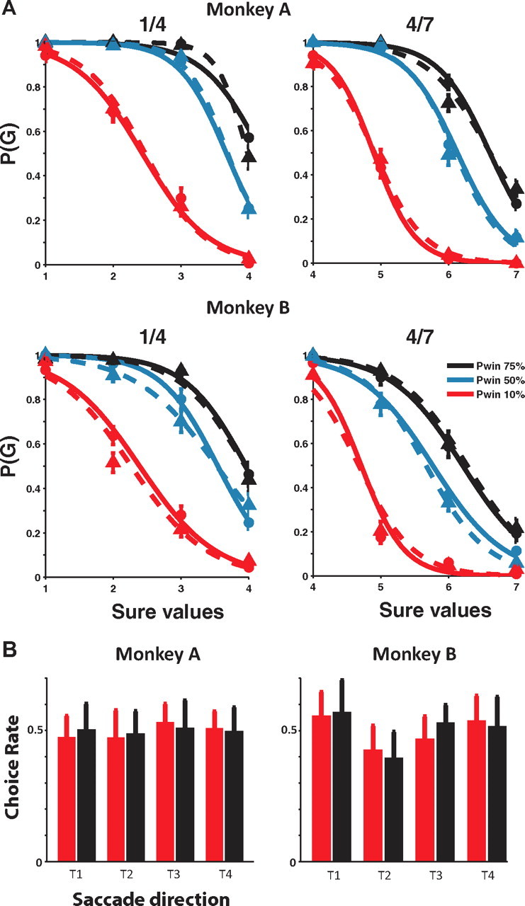
Influence of outcome of previous trial on current choice. A, Choice functions of monkey A (top) and B (bottom), separately drawn depending on the outcome of the previous trial. The solid lines represent the choice curves for the trials after winning trials, and the dotted lines represent the choice curves for the trials after losing trials. The probability that the monkey chooses a particular gamble option [P(G)] is plotted as a function of the value of the alternative sure option. The reward size is indicated as multiples of a minimal reward amount (30 μl). The left column shows gamble options that yield either 30 μl (1 unit) or 160 μl (4 units) with a 10% (red lines), 50% (blue lines), and 75% (black lines) chance of receiving the larger outcome. The right column shows gamble options that yield either 160 μl (4 units) or 210 μl (7 units) with a 10% (red lines), 50% (blue lines), and 75% (black lines) chance of receiving the larger outcome. The figure represents the grand average over all choice trials recorded from monkey A (top row) and B (bottom row). Error bars represent SEM. B, Frequency with which a saccadic direction was chosen after winning (red) or losing (black) a gamble in the previous trial. Both monkeys made a saccade to each of the directions equally often, regardless of the gamble outcome of the previous trial (p > 0.05 for all directions; Bonferroni adjusted).

Behavioral results showed that the monkeys' choices were based upon the relative value of the two options (So and Stuphorn, 2010). The probability of a gamble choice decreased as the alternative sure reward amount increased. In addition, as the probability of receiving the maximum reward (i.e., “winning” the gamble) increased, the monkey showed more preference for the gamble over the sure option. The choice functions allowed us to estimate the subjective value of the gamble to the monkeys in terms of sure reward amounts, independent of the underlying utility functions that relate value to physical outcome. Both monkeys chose the gamble option more often than expected given the probabilities and reward amounts of the outcomes, indicating that the subjective value of the gamble option was larger than its expected value. Thus, the monkeys behaved in a risk-seeking fashion, similar to findings in other gambling tasks using macaques (McCoy and Platt, 2005). The reasons for this tendency, as well as for the general tendency for risk-seeking behavior, are not clear. It might be related to the specific requirements of our experimental setup (i.e., a large number of choices with small stakes). From the point of view of the present experiment, the most important fact is that we can measure the subjective value of the gambles, which is different from the “objective” expected value.

Effects of reinforcement history on choice behavior

The choice of the current trial (gamble or sure) was described by the value of the gamble option, the value of the sure option, and the outcome of the previous trial, such as the following:

where G is the monkey's choice for the current trial (1 for the gamble, and 0 for the sure choice), Vg is the value of the gamble option, Vs is the value of the sure option, and W is the outcome of the previous trial (1 for the win, and 0 for the loss).

Electrophysiology

After training, we placed a square chamber (20 × 20 mm) centered over the midline, 27 mm (monkey A) and 25 mm (monkey B) anterior of the interaural line. During each recording session, single units were recorded using a single tungsten microelectrode with an impedance of 2–4 MΩs (Frederick Haer). The microelectrodes were advanced using a self-build microdrive system. Data were collected using the PLEXON system. Up to four template spikes were identified using principal component analysis and the time stamps were then collected at a sampling rate of 1000 Hz. Data were subsequently analyzed off-line to ensure only single units were included in consequent analyses.

Spike density function

To represent neural activity as a continuous function, we calculated spike density functions by convolving the spike train with a growth-decay exponential function that resembled a postsynaptic potential. Each spike therefore exerts influence only forward in time. The equation describes rate (R) as a function of time (t) as follows:

where τ_g is the time constant for the growth phase of the potential, and τ_d is the time constant for the decay phase. Based on physiological data from excitatory synapses, we used 1 ms for the value of τ_g and 20 ms for the value of τ_d (Sayer et al., 1990).

Task-related neurons

Since we focused our analysis on neuronal activities during delay (after saccade and before result), and result period (from result to reward delivery), we restricted our analyses on the population of neurons active during each of those two periods. We performed t tests on the spike rates in 10 ms intervals throughout the delay and the result period, compared with the baseline activity defined as the average firing rates during the 200–100 ms before target onset. If values of p were <0.05 for five or more consecutive intervals, the cell was classified as task-related in the tested period. Since we treated the results in the two periods as independent, the two different neuronal populations used for further analyses were overlapping, but not identical.

Regression analysis

To quantitatively characterize the modulation of the individual neuron, we designed groups of linear regression models separately for the delay and the result period, using linear combinations of variables that were postulated to describe the neuronal modulation during each time period of interest. In general, we treated the activity in each individual trial as a separate data point for the fitting of the regression models. We analyzed the mean neuronal activity during the first 300 ms after saccade initiation for the early delay period, and the last 300 ms before the result disclosure for the late delay period. For the result period analysis, we used the mean neuronal activity during the first 300 ms after the result disclosure.

Regression analysis for the delay period

To quantitatively identify value (V), uncertainty (U), gamble-exclusive (Vg), and sure-exclusive (Vs) value signals, we built a set of linear regression models having V, G, S, GV, and SV as variables. V represented the subjective value of the option, while G and S were dummy variables indicating whether the saccade target was a gamble or a sure option. GV and SV were the multiplicative term of the variables G and V, and S and V, respectively. Therefore, GV and SV represented gamble-exclusive and sure-exclusive value. Since they were mutually exclusive, we did not cross combine gamble-exclusive (G or GV) and sure-exclusive terms (S or SV) in our regression models. As a result, the following two types of the full model:

were used, along with their respective derivative models. If the best model contained the variable V, we classified the activity as carrying a V signal, as it responded to the value of the chosen option, regardless of whether it was a gamble or a sure option. If either the G or S variable appeared in the best model, we classified the activity as carrying a U signal. Likewise, when the best model contained either GV or SV variable, the activity was classified as carrying a Vg or a Vs signal, respectively. Therefore, a given neuron could be classified as carrying multiple signals.

As noted above, we did not cross-combine gamble- and sure-exclusive terms in Equations 5 and 6. Thus, each class of models served its own purpose independent of the other, albeit at the price of doubling the number of regression models we had to test. To model gamble- or sure-exclusive encoding, we used dummy variables that served as rectifier (1/0). If we had only included gamble/sure choice as a variable, we could have used a single variable. However, in the case of interaction terms (GV and SV), the direction of the rectifier is of importance. This required the use of two complementary sets of regression models.

In our current study, we were interested in whether the SEF neurons contain information about the “chosen” option. Thus, any of the signals identified by the regression analyses described above, should not distinguish between choice and no-choice trials. We therefore tested next whether the neurons showed a significant difference between those two trial types. The best regression model of each cell (determined using the activity from both choice and no-choice trials indiscriminately) was compared against a new model, which was the original best model plus a dummy variable that indicated either a choice or a no-choice trial. If this new model outperformed the original best model, we excluded the neuron from further analyses. This test was performed separately for the early and the late delay period.

Regression analysis for the result period

Reward amount-dependent signals.

To quantitatively classify the various evaluative signals during the result period, we designed two groups of linear regression models. The first set of models was used to describe different types of reward amount-dependent modulation. We identified different types signals represented in neuronal activity according to the best model. If the best model contained the absolute reward amount (R), we identified the activity as carrying a Reward signal. We used two dummy variables to represent a winning (W) or losing (L) trial. If the best model contained any W or L variable, including the interaction terms with R (R*W or R*L), we classified the activity as carrying a Win or a Loss signal, respectively. Similar to the analysis of the delay period activity, we did not cross-combine the winning (W) and losing (L) terms, since they were again mutually exclusive. We therefore tested two different full models and their derivatives as follows:

These two F_W and F_L functions discriminated the two different types of relative reward amount-dependent modulation (F_W for a Win signal, F_L for a Loss signal).

Reward prediction error signals.

The second set of regression models was designed to explain the various types of RPE-dependent modulation. We used four different full models to describe the result period neuronal activity for each trial:

where RPE was defined as follows:

R_actual was the actual reward amount, and R_anticipated was the anticipated reward amount (i.e., the subjective value of each gamble).

In the first two models, RPE_W and RPE_L, respectively, represented the multiplicative interaction term of W (winning) and RPE variable, or L (losing) and RPE. Therefore, if the best model carried either the RPE_W or the RPE_L variable, or their interaction term with R, the neuron was classified as carrying a valence-exclusive RPE signal. We also identified those neurons as carrying Win or Loss signals, respectively. If the best model carried a RPE term or its interaction term with R, we classified this activity as carrying a signed RPE signal (RPEs). Such a neuronal signal reflected both valence and salience of the outcome. Instead, when the best model included an absolute RPE value term (|RPE|), the activity was identified as carrying an unsigned RPE signal (RPEus), and it indicated only salience of the outcome.

A given neuron could be classified as carrying multiple signals. After determining the best model, we tested whether each neuron showed any difference between choice and no-choice trials, using the same procedure we did for the delay period. Those neurons that did were excluded from further analysis.

Encoding of saccade direction

In a previous study (So and Stuphorn, 2010), we analyzed SEF activity during the preparation of the saccadic eye movement. In that paper, we showed that the neurons carried information about the direction of a saccade as well as the anticipated value of the reward. This indicated that SEF neurons encode action value signals, in addition to representing option value. Here, we tested whether the signals following the saccade are still spatially selective and continued to be modulated by the direction of the saccade with which they had chosen the target.

We investigated direction-dependent modulations during the delay period by extending the linear regression model analysis of the SEF neurons. In our previous study, we modeled direction dependency using a circular Gaussian term involving four free parameters. For the current study, we decided to use a more general approach that used fewer assumptions. We therefore modeled direction dependency using four binary variables that indicated the different directions. The full model for these direction-dependent regression models was as follows:

where D₁ was the dummy variable for the most preferred direction, D₂ was the second preferred, D₃ was the third, and finally, D₄ was the least preferred direction. The order of preferred direction was determined from the comparison of the mean neuronal activities for four different directions separately during each time period. Next, for each neuronal activity, the original best model (Orig) was compared against the direction-only model (Dir; which includes the full model g_D and its derivative models), linear (Orig + Dir), and nonlinear (Orig*Dir) combination of the original and the direction model. If any of the directional terms enhanced the fit, the neuron was classified as influenced by direction. In this way, any conceivable pattern of selectivity across the four directions was detected by the analysis.

Coefficient of partial determination

To determine the dynamics of the strength with which the different signals modulated neuronal activity, we calculated the coefficient of partial determination (CPD) for each variable from the mean activity of each neuron during different time bins (50 ms width with 10 ms step size) (Neter et al., 1996). As we had three variables in the full regression model, CPD for each variable (X1) was calculated as follows:

Model fitting

To determine the best fitting regression model, we searched for the model that was the most likely to be correct, given the experimental data. This approach is a statistical method that has its origin in Bayesian data analysis (Gelman et al., 2004). Specifically, we used a form of model comparison, whereby for a pairwise comparison the model with the smaller Bayesian information criterion (BIC) was chosen. For each neuron, a set of BIC values were calculated using the different regression models as follows:

where n was the total trial number, RSS was the residual sum of squares, and K was the number of fitting parameters (Burnham and Anderson, 2002; Busemeyer and Diederich, 2010). A lower numerical BIC value indicates a better fit of a model, since n is constant across all models, a lower RSS indicates better predictive power, and a larger K can be used to penalize less parsimonious models. By comparing all model-dependent BIC values for a given neuron, the best model was determined as the one having the lowest BIC.

This procedure is related to a likelihood-ratio test, and equivalent to choosing a model based on the F statistic (Sawa, 1978). It provides a Bayesian test for nested hypotheses (Kass and Wasserman, 1995). Importantly, we included a baseline model in our set of regression models. Thus, a model with one or more signals was compared against the null hypothesis that none of the signals explained any variance in neuronal activity. An alternative procedure would have been a series of sequential F tests, but this test, while exact, requires the assumption of data with a normal distribution. We decided therefore to use the BIC test, because it was computationally straightforward and potentially more robust. An additional advantage was that we could compare all models simultaneously, using a consistent criterion (Burnham and Anderson, 2002).

Results

Behavior

We trained two monkeys in a gambling task (Fig. 1A), which required them to choose between a sure and a gamble option by making an eye movement to one of two targets. Behavioral results showed that the monkeys' choices were based upon the relative value of the two options (So and Stuphorn, 2010). For each gamble, we plotted the probability of choosing the gamble as a function of the alternative sure reward amount (Fig. 1C). The probability of a gamble choice decreased as the alternative sure reward amount increased. In addition, as the probability of receiving the maximum reward (i.e., “winning” the gamble) increased, the monkey showed more preference for the gamble over the sure option. The choice functions allowed us to estimate the subjective value of the gamble to the monkeys in terms of sure reward amounts, independent of the underlying utility functions that relate value to physical outcome.

To be able to correlate neuronal activity with behavior, it is critical that the monkeys showed the same pattern of preferences throughout a recording session. We computed therefore the monkeys' choice function separately for the first half and the last half of the session of each day (Fig. 1C). Both monkeys showed variability in their choice throughout the session of each day, that is, they preferred sometimes the gamble option and sometimes the sure option, depending on their relative subjective value. Furthermore, there were only small changes in the choice function for the first and second half of each session. This indicates that the monkey's preferences stayed constant across time.

Neuronal data set

We recorded 264 SEF neurons in two monkeys. Of these, 227 cells showed significant activities during the delay period, and 217 cells showed significant activities during the result period. These two groups of task-related neurons were classified independently, and we restricted our analyses of the delay and the result period to those two groups of neurons, respectively. On average, we recorded the cells classified as task-related during the delay period on 941.6 ± 47.5 (SEM) trials. Similarly, 950.6 ± 47.3 trials were recorded on average for each cell we analyzed for the result period. We will first present the neuronal activity during the delay period, and then the activity in the result period.

SEF neurons monitor the choice during the delay period

In our task, the choice was followed by a delay period during which the eventual outcome was not yet known. During this delay period, information about the chosen action needed to be maintained, to correctly evaluate the later outcome. To characterize the neuronal activity, we determined the general linear regression model that best described the activity separately during an early (300 ms after saccade initiation) and a late (300 ms before result onset) section of the delay period. For analysis, we only used the neuronal population showing no difference between choice and no-choice trials [161 neurons (early); 199 neurons (late)].

The most important information regarding the choice is its subjective value (i.e., the reward that is expected to follow from it). We estimated the subjective value of each gamble from the monkey's probability of choosing a gamble as a function of the value of the alternative sure reward option (So and Stuphorn, 2010). During the delay period, many SEF neurons represented the value of the chosen option. Figure 2 shows an example of such a neuron reflecting the subjective value, throughout the early (Fig. 2A) and the late (Fig. 2B) delay period. The regression plots to the right of the histograms show the mean neuronal activity (dots) and the best regression model (lines), against the value of the choice. As we can see, both the early and the late delay neuronal activity represented the value of the choice, regardless of whether it was a sure or a gamble option (V signal). We found 71 such neurons (71 of 161; 44.1%) in the early delay and 42 (42 of 199; 21.1%) in the late delay period.

Figure 2.

An example neuron carrying a value signal during both the early (A) and late (B) delay period. In the spike density histograms, trials are sorted into three groups based on their chosen option value. The black line represents trials with high value (6 units of reward or higher), the dark gray line represents trials with medium value (between 3 and 6 units of reward), and the light gray line represents trials with low value (<3 units of reward). The top row represents the neuronal activities in gamble option trials, and the bottom row represents the neuronal activities in sure option trials. The regression plots to the right of each histogram display the best models (lines) and the mean neuronal activities (dots) during the time periods indicated by the shaded areas in the histograms. The red lines and dots represent gamble option trials, while the blue lines and dots describe sure option trials. Error bars represent SEM.

There was a fundamental difference between sure and gamble options in the degree to which the outcome of a particular choice could be anticipated. Specifically, the outcome of the gamble option was inherently uncertain, and this uncertainty could not be reduced through learning. We found some SEF neurons that encoded this categorical difference between sure and gamble options. An example neuron representing this uncertainty (U) signal is presented in Figure 3A. This neuron showed higher activation for the gamble than for the sure options throughout the whole delay period. The regression plots below the histograms show that the neuronal activity did not reflect the value of different gamble or sure options. Uncertainty signals were more frequent toward the late delay period. We found them in 33 neurons (20.5%) during the early delay period and in 78 neurons (39.2%) during the late delay period.

Figure 3.

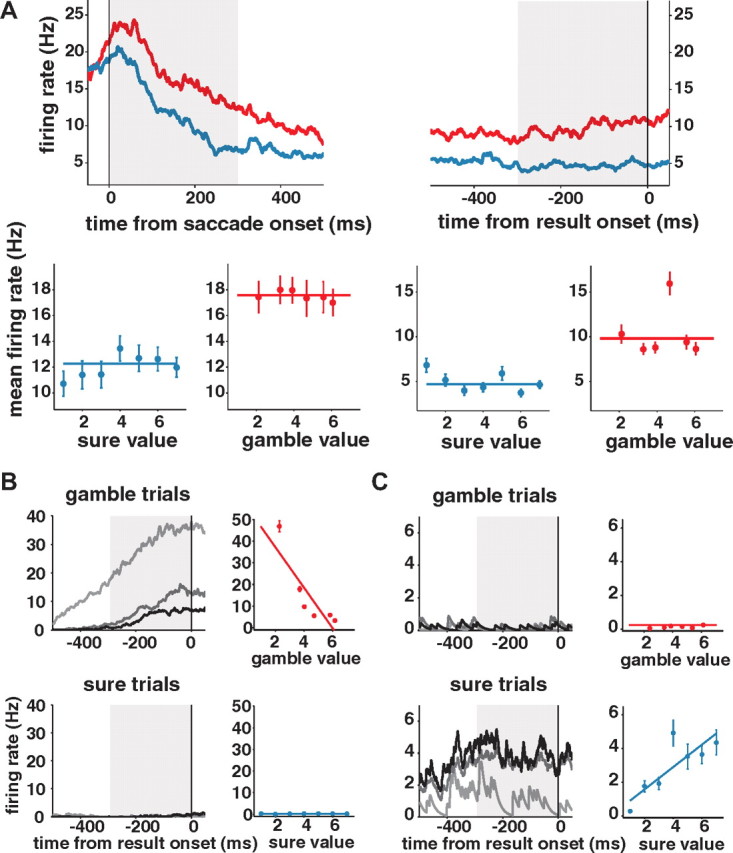
Example neurons carrying uncertainty-related signals during the delay period. A, A neuron representing the categorical uncertainty of the chosen option (U signal) is shown with spike density histogram (top row) and the best regression model (bottom row). This neuron discriminated gamble (red line) and sure option (blue line) throughout early and late delay period. It did not represent the chosen value, as we can see from the best regression model plot in which the average neuronal activity was plotted against different value. B, A neuron representing gamble-exclusive value (Vg signal) is shown with spike density histogram (left) and the best regression model (right). C, A neuron representing Vs signal. For the example neurons for Vg (B) and the Vs (C) signal, only the late delay period activity is shown, as both neurons shown here represented the uncertainty-contingent value signal only in the late delay period. The line and dot colors here follow the convention in Figure 2. Error bars represent SEM.

The difference in uncertainty about the result of gamble and sure options affected the reliability of the value estimates that were associated with those two choices. Accordingly, we also observed SEF neuronal activities, which represented the interaction of the value signal and the categorical uncertainty signal. These reflected value exclusively for the gamble (Vg signal; Fig. 3B) or the sure option (Vs signal; Fig. 3C). Vg and Vs signals were more frequently observed during the late delay period. Vg signals and Vs signals were represented in 27 (16.8%) and 10 neurons (6.2%) during the early delay period, which increased to 42 (21.1%) and 34 neurons (17.1%) in the late delay period, respectively.

Across all neurons, the neuronal activity was more often positively correlated with the value- and uncertainty-related signals (Table 1). Nevertheless, negative correlations were not an uncommon occurrence.

Table 1.

The direction of correlation found in the chosen option-representing neurons during the delay period

	Early			Late
	Pos	Neg	Total	Pos	Neg	Total
V	51	20	71	32	10	42
U	12 (g > s)	21 (s > g)	33	53 (g > s)	25 (s > g)	78
Vg	19	8	27	20	22	42
Vs	7	3	10	31	3	34

Another important piece of information to keep track of during the delay period is the chosen action, here, the saccade direction (So and Stuphorn, 2010). Among the neurons reflecting attributes of the chosen option, a large number of neurons [41% during the early (41 of 101); 45% during the late delay period (62 of 137)] carried also directional information. However, only a minority (1 of 101 during the early; 8 of 137 during the late delay period) represents the directional information alone (Table 2). A χ² test showed no significant dependency between direction-encoding and the original signal(s) carried by a given SEF neuron (p > 0.05 for both early and late delay period). Thus, value and uncertainty information of the chosen option was represented independently of the chosen action (i.e., saccadic direction).

Table 2.

The number of each signal, recounted based upon the saccade direction-included regression analysis

	Early				Late
	V	U	Vg	Vs	V	U	Vg	Vs
Without Dir	71	33	27	10	40	78	41	34
Orig	44	15	15	7	18	40	18	20
Dir only	0	1	1	0	5	5	2	3
Orig + Dir	18	15	9	1	16	28	19	10
Orig*Dir	9	2	2	2	1	5	3	1

Please note that neurons can appear more than once in each column if multiple signals influence the activity of the neuron.

Population dynamics of encoding during delay period

We investigated how SEF neurons dynamically encode these different signals during the delay period using a dynamic regression analysis (50 ms width time bin; 10 ms step size). We first plotted the number of cells that were best described by a model that contained the respective variable at each time point (Fig. 4A). Initially, the subjective value signal (V) dominated the SEF population. However, after ∼100 ms, the number of neurons that represented value sharply dropped, and more neurons started to reflect the uncertainty of the value estimation. Consequently, throughout the late delay period, the uncertainty-related signals (U and Vg, Vs) became more common in the SEF population than the V signal. We also calculated the mean CPD for each variable in the SEF population using the full regression model (Fig. 4B). Similar trends were observed as for the best model analysis. The influence of the V signal on the neuronal activity was predominant immediately after saccade, while the uncertainty-related signals, especially Vg and U, dominated during the later part of the delay period.

Figure 4.

Temporal dynamics of signals representing information about the chosen option. A, The number of cells that include each variable in their best models was counted for each time bin (50 ms width temporal window with 10 ms step). B, Mean CPD for each variable at each time bin. The shaded areas represent SEM.

In sum, the neuronal representation of a chosen option in SEF shows a characteristic development from early to late stages of the delay period. This likely reflects the two distinct decision-making stages that frame the beginning and the end of the delay period, namely, decision execution and its outcome evaluation. The beginning of the delay period, immediately following the decision, is marked by the representation of the value that is expected on the trial. Signals related to the uncertainty of this value estimation start to develop with some delay, and eventually become predominant. These signals are likely more important for the evaluation of the outcome of the choice in the result period.

SEF neurons represent absolute or relative reward amount during result period

On those trials in which the monkey chose the gamble option, the result of the gamble was visually indicated at the beginning of the result period (Fig. 1A). The gamble outcome could be described in absolute terms as the physical reward amount, or in relative terms as a win or loss. Our gambling task allowed us to discriminate between an absolute and a relative outcome signal, by having sets of gamble options with low (1 and 4 units of reward) and high value (4 and 7 units of reward). Therefore, 4 units of reward could mean a win in low value gambles, or a loss in high value gambles.

To quantitatively characterize the activity of SEF neurons during the following result period until reward was physically delivered, we examined the neuronal activities (300 ms after result onset) using linear regression analysis. During this time period, the monkeys still needed to hold the eye position until the reward was actually delivered. The neuronal signals that we describe in the following section are therefore not confounded with the preparation of eye movements following reward delivery. Almost all (213 of 217; 98.2%) of the neurons identified as task-related during the result period did not discriminate between choice and no-choice trials. If the activity of a neuron reflected only the absolute reward amount, the neuron should indicate the amount independent of its context. However, if a neuron reflected the relative reward amount (win/loss), it should show different activity for the same reward amount depending on its context.

In fact, we observed different types of SEF neuronal activity that reflected either absolute or relative reward amount during the result period. Figure 5 shows single neuron examples of each type. The neuron in Figure 5A was modulated only by the absolute reward amount (Reward signal). Figure 5, B and C, shows neurons that were modulated by the relative reward amount. The neuron in Figure 5B increased its activity only when the realized reward amount was the larger one of the two possible outcomes (Win signal). Figure 5C shows the opposite pattern, responding only when the realized reward amount was the smaller one of the two outcomes (Loss signal). Among the 213 task-related neurons, 49 neurons (23%) carried the Reward signals, 41 neurons (19.2%) encoded Win signals, and 45 neurons (21.1%) encoded Loss signals.

Figure 5.

Single-neuron examples representing reward amount during result period. Neuronal activities are sorted by the absolute reward amount [1 (left), 4 (center), and 7 (right) units of reward] and by context (black for loss; red for win). Examples from three different types of reward amount-representing signals are shown. Reward signal reflects the absolute reward amount (A), while Win (B) and Loss signal (C) reflect the different context of reward, winning and losing, respectively. Best regression models, along with the mean neuronal activities, are plotted against the absolute reward amount for each cell, to the right side of the spike density histograms. Error bars represent SEM.

SEF neurons represent reward prediction error during result period

During the delay period, the value of the expected outcome of the trial was represented in many SEF neurons. In addition, during the result period, some SEF neurons encoded the actual reward amount that the monkey was going to receive at the end of the trial. The combination of these two types of signals allows the computation of another type of evaluative signal, namely, the mismatch between the expected and the actual reward amount. This mismatch signal, so-called RPE, is an important signal in reinforcement learning theory, and the monkeys' behavior indicated that they were sensitive to RPE during the result period (Fig. 6).

Figure 6.

Fixation break rates during result period are plotted against the difference between the actual and the anticipated reward (i.e., reward prediction error). The left column represents the results from monkey A, and the right column shows monkey B results. Error bars represent SEM.

We observed four different types of RPE representations (Fig. 7). First, among some cells encoding Win or Loss signals, we observed that the win- or the loss-exclusive activation was also modulated by RPE. For example, the winning-induced activation of the cell shown in Figure 7A was highest when the winning was least expected (gambles with 10% probability to win) (i.e., when the mismatch between actual and expected reward was largest). We will refer to this type of activity as “win-exclusive reward prediction error” (RPE_W) representation. Conversely, the loss-induced activation of the cell in Figure 7B was highest when the losing was least expected (gambles with 75% probability to win). We will refer to this type of activity as “loss-exclusive reward prediction error” (RPE_L) representation. Among 41 neurons encoding Win signals, 20 neurons (48.8%) were additionally modulated by reward prediction error (RPE_W). Likewise, among 45 neurons encoding Loss signals, 15 neurons (33.3%) were additionally modulated by the reward prediction error (RPE_L).

Figure 7.

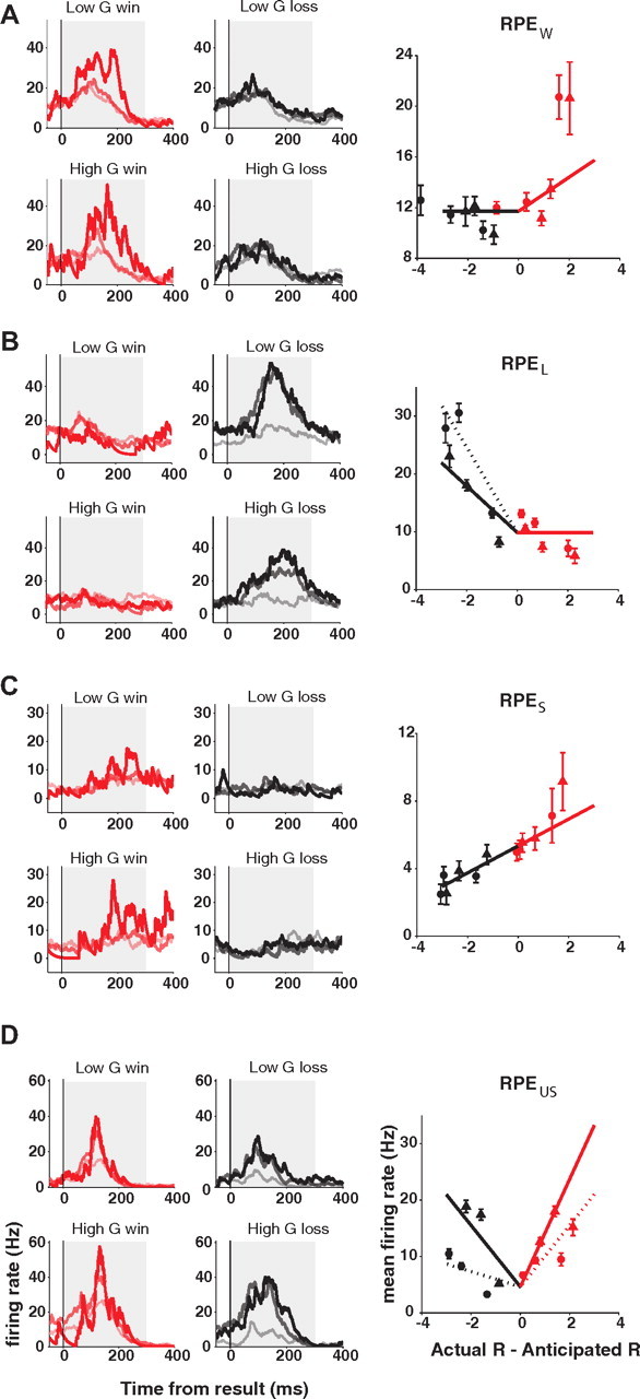
Example neurons carrying different types of RPE signals, representing win-exclusive (RPE_W) (A), loss-exclusive (RPE_L) (B), signed (RPE_S) (C), and unsigned RPE (RPE_US) (D). Spike density histograms for each neuron are plotted separately for low value gamble (top row) and high value gamble (bottom row), and for winning (left, red lines) and losing trials (right, black lines). While different colors represent positive (red) and negative (black) signs, different shades of each color represent the magnitude of RPE. For winning trials, the vivid red line represents the neuronal activity from 10% gambles. As winning is unexpected for gambles with 10% chance of winning, this case holds a high magnitude of RPE. The medium light red line represents 50% gamble winning trials, and the light red line represents 75% gamble winning trials. Likewise, for losing trials, the black line represents the neuronal activity for gambles with 75% chance of winning. The dark gray line represents the winning trials of the 50% gamble, and the light gray line represents the winning trials of the 10% gamble. Best regression models for each neuron (lines), along with the mean neuronal activities (circles for low value gambles; triangles for high value gambles), are plotted against the reward prediction error. In each plot, all lines are derived from the single best-fitting model for each neuron. This model might include other variables, such as the reward amount, in addition to the RPE indicated on the x-axis. In case the best regression model identified an additional modulation by reward amount, a dotted line represents either winning (red dotted line) or losing (black dotted line) for low value gambles, while a solid line represents high value gamble results. When there is no additional modulation by reward amount, a single solid line describes both cases. Error bars represent SEM.

In these first two groups, the RPE representations were contingent on the valence of the outcome. However, we also found some RPE representations in SEF that were not valence exclusive. The neuron shown in Figure 7C is an example. This neuron showed higher activation as the reward prediction error increased and lower activation as the reward prediction error decreased. The modulation faithfully represented the RPE reflecting both valence and salience of an outcome. We will refer to this type of neuronal signal as “signed reward prediction error” (RPE_S). We found 13 cells (13 of 213; 6.1%) representing RPE_S signals. Another type of RPE-sensitive activity in SEF showed modulation depending on the absolute magnitude of RPE, independent of the valence of an outcome. An example of a neuron carrying such a signal is shown in Figure 7D. This neuron showed highest activation when the least expected outcome happened (i.e., winning at 10% gambles or losing at 75% gambles). We will refer to this type of signal as “unsigned reward prediction error” (RPE_US), and it seems to encode only the salience of an outcome. We found 20 cells (20 of 213; 9.4%) representing RPE_US signals.

We also tested whether the SEF activity during the result period encoded saccade direction, using the same analysis as the one used for delay period. In general, we observed a similar result (Table 3). A χ² test showed no significant dependency between direction-encoding and the original signal(s) carried by a given SEF neuron (p = 0.99). Therefore, across the entire SEF population, the direction encoding observed during the result period was independent from the encoding of gamble outcome monitoring and evaluation.

Table 3.

The number of each signal during the result period, recounted based upon the direction-included regression analysis

	R	W	L	RPES	RPEUS	RPEW	RPEL
Without Dir	49	43	42	13	21	20	15
Orig	37	33	33	10	16	16	12
Dir	0	0	0	0	0	0	0
Orig + Dir	12	8	8	3	4	3	2
Orig*Dir	0	2	1	0	1	1	1

Our results therefore suggest that directional information is maintained in SEF neuronal activity in the delay and the result period, although its representation was independent of other monitoring and evaluative signals. This is interesting because it indicates that at the moment when the result of an action is revealed there is a remaining memory signal of the action that was selected. This might simplify certain aspects of reinforcement learning, such as the credit assignment problem (Sutton and Barto, 1998). The fact that value and directional information are represented separately in the population would allow these signals to be used to update the two different value signals found in the SEF (So and Stuphorn, 2010). Specifically, in the case of option-value signals the value evaluation signals could be used separately, while in the case of action-value signals they could be combined with directional information.

Behavioral adjustments by the outcome of the preceding gamble

Reward prediction error alone is not sufficient to lead to the actual learning process, which is indicated by behavioral adjustments (Dayan et al., 2000; Behrens et al., 2007). We therefore tested whether the RPE-related signals in SEF are accompanied by behavioral adjustments. We investigated such possible effects of the outcome of the previous trial on the monkeys' choice in our gambling task using two different ways.

First, we tested whether the choice outcome (win/loss) influenced the likelihood of choosing a gamble. To do so, we analyzed the subset of choice trials, in which the monkey had chosen a gamble option in the previous trial. We fitted the choice curves separately for trials, in which the previous trial was a winning or a losing one (Fig. 8A). Across all six gambles, these two curves showed no significant difference for both monkeys. The distributions of the gamble choices (specifically the frequency with which the gamble was chosen during a particular session) across the individual comparisons of sure and gamble options was also not significantly influenced by outcome history (t tests, p > 0.05, Bonferroni adjusted). Additionally, a linear regression analysis was used to investigate the effect of the outcome of the previous trial on monkeys' choice. For both monkeys, the value of the gamble and the sure option had a highly significant effect on choice (p < 0.00001), while the outcome of the previous trial was not significant (p > 0.05).

Second, we tested whether the choice outcome (win/loss) influenced the spatial direction of the saccade in the next trial. We found that there was no influence of the outcome on the spatial choice of the next trial (Fig. 8B). The frequency of spatial choices was not significantly different after winning or losing a gamble in the previous trial (p > 0.05 for all directions; Bonferroni adjusted). This result is not surprising considering the way our task was designed. In our task, every trial has a different spatial configuration of choice targets, randomly drawn from a set of 12 such configurations. In this way, across all choice trials in the experiment the amount of expected reward should have been allocated equally for each target. This expectation was confirmed by post hoc analysis. Both monkeys experienced on average a similar amount of reward from each of the quadrants (monkey A: T1, 4.20 ± 0.16; T2, 4.32 ± 0.20; T3, 4.57 ± 0.16; T4, 4.52 ± 0.17 reward units; monkey B: T1, 4.27 ± 0.14; T2, 4.83 ± 0.21; T3, 4.52 ± 0.13; T4, 4.29 ± 0.12 reward units; errors are in SD). This implied that there were no environmental contingencies that could drive the development of spatial biases. Consequently, the monkeys made eye movements to each quadrant approximately equally often (Fig. 8B).

Discussion

SEF monitors choices and evaluates their outcome

Following any choice, the most important variable to monitor is the estimated value of the chosen option, since it drove the selection process. Accordingly, SEF neurons represent the expected value of the chosen option throughout the entire delay period. Following decisions under risk, the outcome is uncertain and it becomes important to monitor the presence and amount of this uncertainty as well.

However, the uncertainty signals in SEF emerge only later in the delay period; hence, they are clearly not involved in decision making. Instead, they likely serve to modulate the outcome evaluation. Theoretical models have suggested that it would be useful to track prediction risk (i.e., the expected size of a prediction error) (Yu and Dayan, 2005; Preuschoff and Bossaerts, 2007), as it could be used to optimize the reaction to the prediction error. The SEF uncertainty signal could track prediction risk as required by these models. Uncertainty signals observed in midbrain dopamine neurons, anterior insular cortex, and striatum (Fiorillo et al., 2003; Preuschoff et al., 2006) show a similar dynamics as the one in SEF, appearing later than value-encoding signals. These brain regions are closely connected and might form a functional network.

During the result period, SEF neurons represented the actual reward. This is critical because outcome evaluation depends on the comparison of both expected and actual reward. This reward signal often indicated the relative (Win or Loss) rather than the absolute reward amount. Similar relative reward encoding was also found in other reward-related brain areas, such as midbrain dopamine nuclei (Tobler et al., 2005), habenula (Matsumoto and Hikosaka, 2009a), orbitofrontal (Tremblay and Schultz, 1999), and medial frontal cortex (Seo and Lee, 2009). However, this neuronal activity is contingent on the valence of the outcome and is therefore not suitable to generate the whole range of a reward prediction error signal, in contrast to the neuronal activity representing absolute reward amount.

We observed four different RPE representations in SEF during the result period. The RPE_S signal reflected both valence and salience of the outcome. Such a RPE_S signal is equivalent to the teaching signal that is predicted in the Rescorla–Wagner model of reinforcement learning (Rescorla and Wagner, 1972), and is similar to the well known signal carried by midbrain dopamine and habenular neurons (Schultz et al., 1997; Matsumoto and Hikosaka, 2007). However, the RPE_US signal is equivalent to the salience signal that is predicted in the Pearce–Hall model of reinforcement learning. In this model, the salience signal controls the amount of attention that is paid to a task event and thus indirectly the amount of learning (Pearce and Hall, 1980). Recently, it has been reported that some dopaminergic neurons in the midbrain encode a valence-independent salience signal (Matsumoto and Hikosaka, 2009b). If confirmed, such a salience signal would be similar to the RPE_US signal we report here in SEF. A similar salience-related RPE signal was also reported in the amygdala of macaques (Belova et al., 2007) and rats (Roesch et al., 2010), as well as in the basal forebrain of rats (Lin and Nicolelis, 2008).

In addition, many SEF neurons encoded reward prediction error selectively for outcomes of a specific valence (RPE_W and RPE_L signals). A very similar valence-specific RPE signal was also found in the amygdala (Belova et al., 2007) and in the ACC (Matsumoto et al., 2007) of primates. An important difference between our study and others is that we did not use aversive stimuli, such as air puffs. It is therefore an open question whether the Loss-specific activities in the SEF that responded to the smaller reward would also respond to a true aversive stimulus. While this is a question that needs to be resolved empirically, the monkeys may have indeed regarded lost gambles as aversive outcomes. This interpretation was supported by the observation that both monkeys' fixation break rate was significantly higher for lost gamble trials, even though fixation breaks at the end of the trial were very costly to the monkeys.

Functional architecture of outcome evaluation

Our findings in SEF fit well into a new emerging picture of how outcomes are evaluated by the brain. First, in our SEF population, as well as in dopaminergic midbrain neurons and in the amygdala, various valence- and salience-based evaluative signals coexist in neighboring groups of neurons. The wide distribution of brain regions in which valence-independent salience signals are found suggests a ubiquitous presence of this type of evaluative signal. This heterogeneous mixture of signals suggests that the current understanding of reinforcement learning, which has been largely based upon the Rescorla–Wagner model (Rescorla and Wagner, 1972), needs to be expanded by including motivational saliency (Pearce and Hall, 1980). In fact, a hybrid learning model has been developed (LePelley, 2004).

Second, our findings also support long-standing theoretical ideas regarding the evaluation of affective states by two separate processes (Konorski, 1967; Solomon and Corbit, 1974). The neuronal systems processing appetitive and aversive stimuli closely interact, which might explain the heterogeneous representation present in SEF. These heterogeneous signals can control behavior in different ways. On the one hand, appetitive and aversive signals might act in an opponent manner, as in valence-dependent RPE representations. These signals could be used to directly adjust action value representations in SEF (Seo and Lee, 2009; So and Stuphorn, 2010) and in this way could influence the future allocation of behavior. Alternatively, appetitive and aversive signals might act in a congruent manner, as in salience-dependent RPE representations. The motivational salience of events is related to their ability to capture attention (Holland and Gallagher, 1999). The role of the SEF in attention is not very well understood, but SEF is known to be active in attentional tasks (Kastner et al., 1999). It is therefore possible that the valence-independent salience signals in the SEF serve to guide attention toward motivationally important events.

Our current gambling task design does not promote behavioral adjustments. It is therefore interesting to note that we found the neuronal correlates of RPE signals even without the need for behavioral adjustments. RPE alone does not necessarily lead to learning. The learning process also requires a nonzero learning rate, which is determined by the statistics of the environment (i.e., volatility) (Dayan et al., 2000; Behrens et al., 2007). This disassociation suggests that the process of learning and the (potentially automatic) process of RPE computation might be separated.

Origin of reward prediction error signals

Outcome-related neuronal activities are found in a very large network of areas. This poses the question of the relationship of these signals to similar RPE signals in other brain structures. Our findings suggest that, in the case of eye movements, the SEF could compute the RPE signals locally without input from other structures. In that case, the SEF might send those RPE signals to the amygdala (Ghashghaei et al., 2007), as well as to the dopaminergic midbrain nuclei and the habenula via connections through the basal ganglia. The SEF projects to the striatum, which projects to the dopaminergic midbrain nuclei (Calzavara et al., 2007) and to the habenula (Hong and Hikosaka, 2008). Local computation of RPE may happen in parallel in other brain structures, as suggested by recent studies in orbitofrontal cortex (Sul et al., 2010), striatum (Kim et al., 2009), and ACC (Seo and Lee, 2007). More general signals might be generated through converging inputs from multiple specialized evaluation systems onto a central, general node, such as the midbrain dopamine and the habenula neurons.

However, we cannot rule out the possibility that SEF might passively reflect the outcome-related signals coming from other areas. In addition to the projections from frontal cortex, the amygdala also projects back to frontal cortex, including SEF (Ghashghaei et al., 2007). Likewise, the SEF, together with other parts of the medial frontal cortex, receives a dense dopaminergic projection (Schultz, 1998; Holroyd and Coles, 2002). It will require additional experiments to test which of these possibilities is correct. For example, it would be useful to study other brain regions using our gambling task, to describe the relative timing of different outcome-related signals.

Conclusion

Our results show that SEF neurons carry various monitoring and evaluative signals in a task that requires decision making under uncertainty. These findings provide a new understanding of the role of SEF in the evaluation of value-based decision making. First, the SEF contains all signals necessary to compute RPE signals and is therefore in a position to independently evaluate the outcome of saccadic behavior. Second, the evaluative signals in SEF support both reinforcement learning models that rely on valence-sensitive and those that rely on valence-insensitive RPE signals. This finding matches recent results in other brain regions and suggests the need for hybrid models of reinforcement learning. Third, the sheer number of different evaluative signals found in SEF is remarkable. It will be important to test other parts of the medial frontal cortex with similar tasks to determine whether this finding is specific to SEF or a more general characteristic of medial frontal cortex and potentially also of other brain regions.

References

- Amador N, Schlag-Rey M, Schlag J. Reward-predicting and reward-detecting neuronal activity in the primate supplementary eye field. J Neurophysiol. 2000;84:2166–2170. doi: 10.1152/jn.2000.84.4.2166. [DOI] [PubMed] [Google Scholar]
- Behrens TE, Woolrich MW, Walton ME, Rushworth MF. Learning the value of information in an uncertain world. Nat Neurosci. 2007;10:1214–1221. doi: 10.1038/nn1954. [DOI] [PubMed] [Google Scholar]
- Belova MA, Paton JJ, Morrison SE, Salzman CD. Expectation modulates neural responses to pleasant and aversive stimuli in primate amygdala. Neuron. 2007;55:970–984. doi: 10.1016/j.neuron.2007.08.004. [DOI] [PMC free article] [PubMed] [Google Scholar]
- Burnham KP, Anderson DR. Model selection and multimodal inference. New York: Springer; 2002. [Google Scholar]
- Busemeyer JR, Diederich A. Cognitive modeling. Thousand Oaks, CA: Sage; 2010. [Google Scholar]
- Calzavara R, Mailly P, Haber SN. Relationship between the corticostriatal terminals from areas 9 and 46, and those from area 8A, dorsal and rostral premotor cortex and area 24c: an anatomical substrate for cognition to action. Eur J Neurosci. 2007;26:2005–2024. doi: 10.1111/j.1460-9568.2007.05825.x. [DOI] [PMC free article] [PubMed] [Google Scholar]
- Dayan P, Kakade S, Montague PR. Learning and selective attention. Nat Neurosci. 2000;3(Suppl):1218–1223. doi: 10.1038/81504. [DOI] [PubMed] [Google Scholar]
- Fiorillo CD, Tobler PN, Schultz W. Discrete coding of reward probability and uncertainty by dopamine neurons. Science. 2003;299:1898–1902. doi: 10.1126/science.1077349. [DOI] [PubMed] [Google Scholar]
- Gelman A, Carlin JB, Stern HS, Rubin DB. Bayesian data analysis. Ed 2. Boca Raton, FL: Chapman and Hall/CRC; 2004. [Google Scholar]
- Ghashghaei HT, Hilgetag CC, Barbas H. Sequence of information processing for emotions based on the anatomic dialogue between prefrontal cortex and amygdala. Neuroimage. 2007;34:905–923. doi: 10.1016/j.neuroimage.2006.09.046. [DOI] [PMC free article] [PubMed] [Google Scholar]
- Hayden BY, Nair AC, McCoy AN, Platt ML. Posterior cingulate cortex mediates outcome-contingent allocation of behavior. Neuron. 2008;60:19–25. doi: 10.1016/j.neuron.2008.09.012. [DOI] [PMC free article] [PubMed] [Google Scholar]
- Holland PC, Gallagher M. Amygdala circuitry in attentional and representational processes. Trends Cogn Sci. 1999;3:65–73. doi: 10.1016/s1364-6613(98)01271-6. [DOI] [PubMed] [Google Scholar]
- Holroyd CB, Coles MG. The neural basis of human error processing: reinforcement learning, dopamine, and the error-related negativity. Psychol Rev. 2002;109:679–709. doi: 10.1037/0033-295X.109.4.679. [DOI] [PubMed] [Google Scholar]
- Hong S, Hikosaka O. The globus pallidus sends reward-related signals to the lateral habenula. Neuron. 2008;60:720–729. doi: 10.1016/j.neuron.2008.09.035. [DOI] [PMC free article] [PubMed] [Google Scholar]
- Huerta MF, Kaas JH. Supplementary eye field as defined by intracortical microstimulation: connections in macaques. J Comp Neurol. 1990;293:299–330. doi: 10.1002/cne.902930211. [DOI] [PubMed] [Google Scholar]
- Kass RE, Wasserman L. A reference Bayesian test for nested hypotheses and its relationship to the Schwarz criterion. J Am Stat Assoc. 1995;90:928–934. [Google Scholar]
- Kastner S, Pinsk MA, De Weerd P, Desimone R, Ungerleider LG. Increased activity in human visual cortex during directed attention in the absence of visual stimulation. Neuron. 1999;22:751–761. doi: 10.1016/s0896-6273(00)80734-5. [DOI] [PubMed] [Google Scholar]
- Kim H, Sul JH, Huh N, Lee D, Jung MW. Role of striatum in updating values of chosen actions. J Neurosci. 2009;29:14701–14712. doi: 10.1523/JNEUROSCI.2728-09.2009. [DOI] [PMC free article] [PubMed] [Google Scholar]
- Konorski J. Integrative activity of the brain: an interdisciplinary approach. Chicago; London: University of Chicago; 1967. [Google Scholar]
- LePelley ME. The role of associative history in models of associative learning: a selective review and a hybrid model. Q J Exp Psychol. 2004;57:193–243. doi: 10.1080/02724990344000141. [DOI] [PubMed] [Google Scholar]
- Lin SC, Nicolelis MA. Neuronal ensemble bursting in the basal forebrain encodes salience irrespective of valence. Neuron. 2008;59:138–149. doi: 10.1016/j.neuron.2008.04.031. [DOI] [PMC free article] [PubMed] [Google Scholar]
- Luce RD. Utility of gains and losses: measurement-theoretical and experimental approaches. Mahwah, NJ: Erlbaum; 2000. [Google Scholar]
- Matsumoto M, Hikosaka O. Lateral habenula as a source of negative reward signals in dopamine neurons. Nature. 2007;447:1111–1115. doi: 10.1038/nature05860. [DOI] [PubMed] [Google Scholar]
- Matsumoto M, Hikosaka O. Representation of negative motivational value in the primate lateral habenula. Nat Neurosci. 2009a;12:77–84. doi: 10.1038/nn.2233. [DOI] [PMC free article] [PubMed] [Google Scholar]
- Matsumoto M, Hikosaka O. Two types of dopamine neuron distinctly convey positive and negative motivational signals. Nature. 2009b;459:837–841. doi: 10.1038/nature08028. [DOI] [PMC free article] [PubMed] [Google Scholar]
- Matsumoto M, Matsumoto K, Abe H, Tanaka K. Medial prefrontal cell activity signaling prediction errors of action values. Nat Neurosci. 2007;10:647–656. doi: 10.1038/nn1890. [DOI] [PubMed] [Google Scholar]
- McCoy AN, Platt ML. Risk-sensitive neurons in macaque posterior cingulate cortex. Nat Neurosci. 2005;8:1220–1227. doi: 10.1038/nn1523. [DOI] [PubMed] [Google Scholar]
- Nakamura K, Roesch MR, Olson CR. Neuronal activity in macaque SEF and ACC during performance of tasks involving conflict. J Neurophysiol. 2005;93:884–908. doi: 10.1152/jn.00305.2004. [DOI] [PubMed] [Google Scholar]
- Neter J, Kutner MH, Nachtsheim CJ, Wasserman W. Applied linear statistical models. Ed 4. Boston: McGraw-Hill; 1996. [Google Scholar]
- Pearce JM, Hall G. A model for Pavlovian learning: variations in the effectiveness of conditioned but not unconditioned stimuli. Psychol Rev. 1980;87:532–552. [PubMed] [Google Scholar]
- Preuschoff K, Bossaerts P. Adding prediction risk to the theory of reward learning. Ann N Y Acad Sci. 2007;1104:135–146. doi: 10.1196/annals.1390.005. [DOI] [PubMed] [Google Scholar]
- Preuschoff K, Bossaerts P, Quartz SR. Neural differentiation of expected reward and risk in human subcortical structures. Neuron. 2006;51:381–390. doi: 10.1016/j.neuron.2006.06.024. [DOI] [PubMed] [Google Scholar]
- Rescorla RA, Wagner AR. A theory of Pavlovian conditioning: variations in the effectiveness of reinforcement and nonreinforcement. In: Black AH, Prokasy WF, editors. Classical conditioning II: Current research and theory. New York: Appleton-Century-Crofts; 1972. pp. 64–99. [Google Scholar]
- Roesch MR, Calu DJ, Esber GR, Schoenbaum G. Neural correlates of variations in event processing during learning in basolateral amygdala. J Neurosci. 2010;30:2464–2471. doi: 10.1523/JNEUROSCI.5781-09.2010. [DOI] [PMC free article] [PubMed] [Google Scholar]
- Sawa T. Information criteria for discriminating among alternative regression models. Econometrica. 1978;46:1273–1291. [Google Scholar]
- Sayer RJ, Friedlander MJ, Redman SJ. The time course and amplitude of EPSPs evoked at synapses between pairs of CA3/CA1 neurons in the hippocampal slice. J Neurosci. 1990;10:826–836. doi: 10.1523/JNEUROSCI.10-03-00826.1990. [DOI] [PMC free article] [PubMed] [Google Scholar]
- Schultz W. Predictive reward signal of dopamine neurons. J Neurophysiol. 1998;80:1–27. doi: 10.1152/jn.1998.80.1.1. [DOI] [PubMed] [Google Scholar]
- Schultz W, Dayan P, Montague PR. A neural substrate of prediction and reward. Science. 1997;275:1593–1599. doi: 10.1126/science.275.5306.1593. [DOI] [PubMed] [Google Scholar]
- Seo H, Lee D. Temporal filtering of reward signals in the dorsal anterior cingulate cortex during a mixed-strategy game. J Neurosci. 2007;27:8366–8377. doi: 10.1523/JNEUROSCI.2369-07.2007. [DOI] [PMC free article] [PubMed] [Google Scholar]
- Seo H, Lee D. Behavioral and neural changes after gains and losses of conditioned reinforcers. J Neurosci. 2009;29:3627–3641. doi: 10.1523/JNEUROSCI.4726-08.2009. [DOI] [PMC free article] [PubMed] [Google Scholar]
- So NY, Stuphorn V. Supplementary eye field encodes option and action value for saccades with variable reward. J Neurophysiol. 2010;104:2634–2653. doi: 10.1152/jn.00430.2010. [DOI] [PMC free article] [PubMed] [Google Scholar]
- Solomon RL, Corbit JD. An opponent-process theory of motivation. I. Temporal dynamics of affect. Psychol Rev. 1974;81:119–145. doi: 10.1037/h0036128. [DOI] [PubMed] [Google Scholar]
- Stuphorn V, Taylor TL, Schall JD. Performance monitoring by the supplementary eye field. Nature. 2000;408:857–860. doi: 10.1038/35048576. [DOI] [PubMed] [Google Scholar]
- Stuphorn V, Brown JW, Schall JD. Role of supplementary eye field in saccade initiation: executive, not direct, control. J Neurophysiol. 2010;103:801–816. doi: 10.1152/jn.00221.2009. [DOI] [PMC free article] [PubMed] [Google Scholar]
- Sul JH, Kim H, Huh N, Lee D, Jung MW. Distinct roles of rodent orbitofrontal and medial prefrontal cortex in decision making. Neuron. 2010;66:449–460. doi: 10.1016/j.neuron.2010.03.033. [DOI] [PMC free article] [PubMed] [Google Scholar]
- Sutton RS, Barto AG. Reinforcement learning. Cambridge, MA: MIT; 1998. [Google Scholar]
- Tobler PN, Fiorillo CD, Schultz W. Adaptive coding of reward value by dopamine neurons. Science. 2005;307:1642–1645. doi: 10.1126/science.1105370. [DOI] [PubMed] [Google Scholar]
- Tremblay L, Schultz W. Relative reward preference in primate orbitofrontal cortex. Nature. 1999;398:704–708. doi: 10.1038/19525. [DOI] [PubMed] [Google Scholar]
- Yu AJ, Dayan P. Uncertainty, neuromodulation, and attention. Neuron. 2005;46:681–692. doi: 10.1016/j.neuron.2005.04.026. [DOI] [PubMed] [Google Scholar]