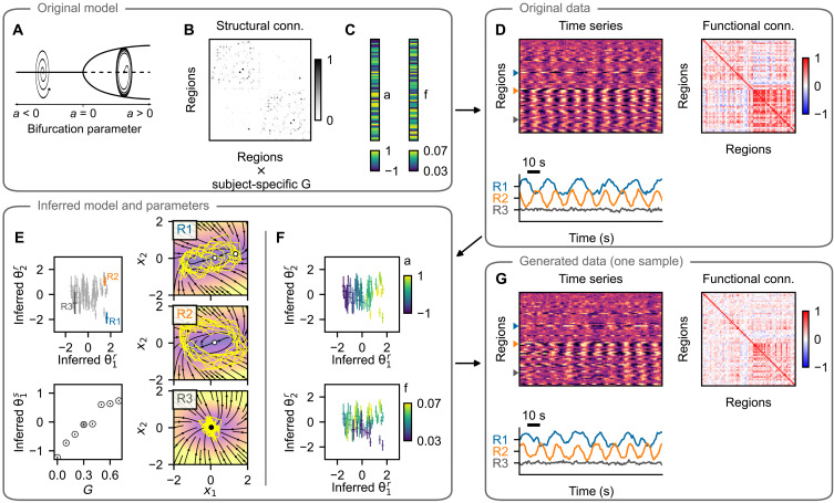
Fig. 2. Hopf model test case: example subject.

(A) The training data are simulated using a network model of brain dynamics, where, in each node, a Hopf neural mass model is placed. (B) The nodes are coupled through a connectome derived from diffusion-weighted imaging scaled by a subject-specific coupling parameter G. (C) The values of bifurcation parameter a_i and intrinsic frequency f_i vary across brain regions. (D) Time series generated with the original model with three examples (bottom) and the calculated FC (right). (E) Inferred regional parameters for all regions (top left; example nodes highlighted) and inferred subject-specific parameter (bottom left; in gray among parameters for all subjects in the dataset). The span of the crosses/lines corresponds to two SDs of the inferred Gaussian distribution. Bottom: Circles are added for visual aid because of the small SDs. The inferred dynamics in state space of the three example nodes are on the right. The vector field is evaluated assuming zero network input and the inferred parameters. Background color, velocity magnitude; yellow lines, exemplary simulated time series of the node activity; Black- and white-faced circles, stable and unstable fixed points. In the topmost panel, an unstable fixed point and a stable fixed point are visually overlapping. (F) Inferred regional parameters colored by the ground truth values of the bifurcation parameter a_i (top) and frequency f_i (bottom). The bifurcation parameter correlates with inferred ${\mathrm{\theta }}_2^r$, while frequency correlates with ${\mathrm{\theta }}_1^r$, but only for regions in the oscillatory regime, i.e., where a_i > 0. (G) One example of the time series generated with the trained model and using the inferred parameters. Important features of the data are preserved both on the regional level (amplitude and frequency) and on the network level (FC).