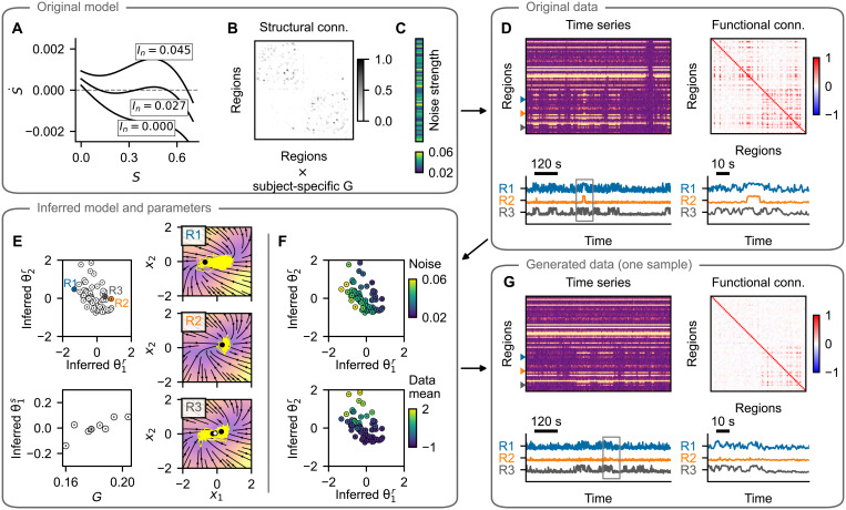
Fig. 3. pMFM test case: example subject.

Layout is the same as in Fig. 2. (A to C) The training data are simulated using a network of pMFM neural masses. Depending on the network input, these can be forced into the monostable regime (down- or up-state) or into the bistable regime. The dynamics is noise driven, with noise strength varying across regions. (D) Time series generated with the original model and the FC. Three examples are shown in the bottom panel, with a window of 100 s on the right. (E) Inferred regional parameters (top left) and subject-specific parameter. Circles are added for visual aid because of the small SDs. The inferred dynamics in state space of the three example nodes are on the right. The vector field is evaluated assuming network input u = 1 and using the inferred parameters. Background color, velocity magnitude; yellow lines, exemplary simulated time series of the node activity; black- and white-faced circles, stable and unstable fixed points. (F) Inferred regional parameters colored by the ground truth values of the noise strength parameter (top). The original parameter is stored along the diagonal of the inferred parameter space. Bottom: Coloring according to the mean of the original time series, which does not represent an original model parameter, rather a data feature. (G) One example of the time series generated with the trained model and using the inferred parameters. Region-specific features (switching between states and noisiness) are well preserved. Structure of the regional correlations is also reproduced, but the correlations are weaker compared to the original. Note that even if the regional time series exhibit signs of bistability (up- and down-state), this bistability may arise at the network level and not necessarily at the regional level, as evidenced by the phase plots in (E).