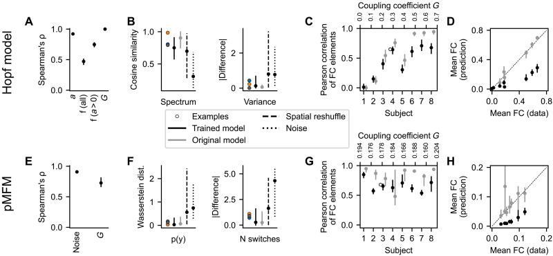
Fig. 4. Quantitative evaluation of the synthetic test cases.

Top row: Hopf model. Bottom row: pMFM. (A and E) Nonlinear correlation between the original parameters and the optimal projection of the inferred region-specific parameters (bifurcation parameter a and frequency f for Hopf model and noise strength for pMFM) and subject-specific parameter (coupling strength G). (B and F) Fit between the regional features of the original time series and those generated by the trained model. We show the cosine similarity of the time series spectra and the difference in variance for the Hopf model and Wasserstein distance of the distributions in the observation space and the difference in logarithm of number of switches for pMFM. These are evaluated for the examples from Figs. 2 and 3, all time series generated by the trained model, and the surrogates described in the main text. (C and G) Fit between the FC of the original and generated time series. (D and H) Mean value of nondiagonal elements of FC matrices. For both models, the correlation strength is underestimated, even if the structure is preserved. In all panels, the bars show the (5, 95) percentile interval with the dot representing the median value. The statistics are computed from 50 samples of the posterior distribution for eight subjects [grouped together in (A), (B), (E), and (F)] and 68 regions (for region-specific parameters and features). The statistics of the surrogate distributions using the original model are also calculated from 50 samples.