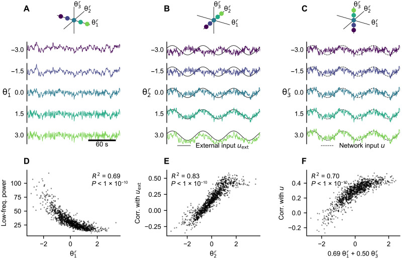
Fig. 7. Effect of the regional parameters on the generated data.

(A to C) With the trained model, we simulate the time series of a single region while varying one regional parameter. In each panel, we systematically vary one of the region-specific parameters while keeping others set to zero. The system and observation noise are generated randomly from standard normal distributions but kept the same for all simulations. In (A), the external input and network input are set to zero. In (B), the external input is set to a sine wave with frequency of 0.014 Hz and the network input is set to zero. In (C), the external input is set to zero and the network input is set to a sine wave with frequency of 0.014 Hz. (D to F) Statistical analysis of the parameter effects illustrated in (A) to (C). We repeatedly (n = 1000) simulated the dynamics of a single region with randomly selected θ^r (see main text). (D) Relation of the low-frequency power (below 0.1 Hz) and ${\mathrm{\theta }}_1^r$. (E) Relation of the Pearson correlation coefficient of the generated time series with the network input u_ext and ${\mathrm{\theta }}_2^r$. (F) Relation of the Pearson correlation coefficient of the generated time series with the network input u and the linear combination of ${\mathrm{\theta }}_1^r$ and ${\mathrm{\theta }}_3^r$ identified by a multivariate regression (fig. S13).