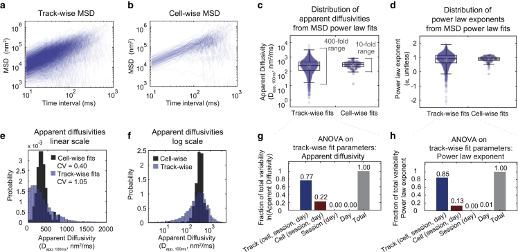
Figure 2.
GEM diffusivity varies over 400-fold across tracks and 10-fold across cells. (a and b) MSDs averaged either (a) by track (averaged over time for each track) or (b) by cell (averaged over time for each track and then averaged across all tracks in each cell). Note the logarithmic scale along the x and y axes. (c and d) Apparent diffusivities (c) and power law exponents (d) calculated from fits of the track-wise and cell-wise MSDs to a power law. Note the logarithmic scale along the y axis. Boxplots: central line, median; gray dot, mean; boxes, 25th and 75th percentiles; whiskers, furthest data points that are not an outlier; outliers, any point that is more than 1.5 times the interquartile-range past the 25th and 75th percentiles. (e and f) The same distributions of the fitted apparent diffusivities plotted in (c), now plotted as a histogram either on a linear scale (e) or on a log scale (f). Probabilities represent the probability density per histogram bin width, such that the sum of the bin heights multiplied by the bin width equals 1. (g and h) Results from a nested ANOVA performed on track-wise fits of diffusivities (g) and power law exponents (h). The amount of the experimentally observed variance that can be explained by track-to-track, cell-to-cell, imaging session-to-session, and day-to-day variability is plotted as a fraction of the total variance. (a–h) The data set is identical to that shown in Fig. 1, c–f, including 3681 tracks among 145 cells, recorded from 5 different samples and over 3 different days.

