

Abstract
Background:
4D Flow MRI is a quantitative imaging technique to evaluate blood flow patterns, however it is unclear how compressed sensing (CS) acceleration would impact aortic hemodynamic quantification in type B aortic dissection (TBAD).
Purpose:
To investigate CS-accelerated 4D Flow MRI performance compared to GRAPPA-accelerated 4D Flow MRI (GRAPPA) to evaluate aortic hemodynamics in TBAD.
Study Type:
Prospective.
Population:
12 TBAD patients, 2 volunteers.
Field Strength/Sequence:
1.5T, 3D time-resolved cine phase-contrast gradient echo sequence.
Assessment:
GRAPPA (acceleration factor [R] = 2) and two CS-accelerated (R = 7.7 [CS7.7] and 10.2 [CS10.2]) 4D Flow MRI scans were acquired twice for interscan reproducibility assessment. Voxelwise kinetic energy (KE), peak velocity (PV), forward flow (FF), reverse flow (RF) and stasis were calculated. Plane-based mid-lumen flows were quantified. Imaging times were recorded.
Tests:
Repeated measures analysis of variance, Pearson correlation coefficients (r), intraclass correlation coefficients (ICC). P < 0.05 indicated statistical significance.
Results:
The KE and FF in true lumen (TL) and PV in false lumen (FL) did not show difference among three acquisition types (p = 0.818, 0.065, 0.284 respectively). The PV and stasis in TL were higher, KE, FF and RF in FL were lower, and stasis was higher in GRAPPA compared to CS7.7 and CS10.2. The RF was lower in GRAPPA compared to CS10.2. The correlation coefficients were strong in TL (r = [0.781 – 0.986]), and low to strong in FL (r = [0.347 – 0.948]). The ICC levels demonstrated moderate to excellent interscan reproducibility (0.732 – 0.989). The FF and net flow in mid-descending aorta TL were significantly different between CS7.7 and CS10.2.
Conclusion:
CS-accelerated 4D Flow MRI has potential for clinical utilization with shorter scan times in TBAD. Our results suggest similar hemodynamic trends between acceleration types, but CS-acceleration impacts KE, FF, RF and stasis more in FL.
Keywords: 4D Flow, MRI, aorta, dissection, hemodynamics, flow
INTRODUCTION
Aortic dissection results from a tear in the aortic intima forming a second blood filled channel known as a false lumen (FL) parallel to the native aortic channel (true lumen [TL]) (1, 2). Aortic dissection can be associated with acute hemodynamic compromise and serious adverse outcomes with morbidity and mortality rates depending on its subtype and extent (3, 4). Stanford type A aortic dissection (TAAD) occurs when a tear develops in the ascending aorta creating a FL and is considered as a surgical emergency (3, 5). Dissection in the descending aorta can occur in isolation (de novo type B aortic dissection [dnTBAD]), or as a residual chronic dissection following TAAD repair (rTAAD) (6, 7). Uncomplicated TBAD without end organ ischemia or rupture is managed medically with anti-impulse therapy (8, 9). However, 20–50% of medically managed chronic TBAD patients eventually require surgical intervention during their clinical follow-up (6, 8, 10–12). It is therefore important to determine which patients will benefit from early surgical intervention such as thoracic endovascular repair (TEVAR), graft replacement or open elephant trunk repair (ET) (13, 14). Considering all these variables, noninvasive imaging is important for diagnosis, risk stratification and selection and accurate timing of the treatment method in TBAD cases.
Three-dimensional time-resolved cine phase-contrast MRI, also known as ‘4D Flow MRI’, has increased clinical utilization over the past several decades and can be used to evaluate several cardiovascular pathologies including aortic stenosis, bicuspid aortic valve disease, aortic coarctation, and aortic dissection (1, 6, 15–19). It has more recently been used to identify TBAD patients with growing aortas at risk for adverse outcomes by assessing the blood flow at entry tears and in the FL (19–25). However, its clinical adoption is hindered by relatively long scan times, especially in critically ill TBAD patients. Thus, a need exists for validation of accelerated 4D Flow MRI protocols in TBAD.
Compressed sensing (CS) acceleration utilizes the inherent sparsity of MRI data and has been combined with various parallel imaging techniques to accelerate MRI acquisitions over the past decade, including 4D Flow MRI (26–30). Even though the results of previous studies have shown improvements in scan time compared to parallel imaging methods, implementation of this technique into clinical workflows has been hindered by long offline reconstruction times (26–28, 30–32). Ma et al recently demonstrated the feasibility of CS-accelerated 4D Flow MRI with inline image reconstruction to obtain thoracic aorta images in under 2 minutes (30). However, while nine different acceleration factor (R) levels were used to evaluate the CS-accelerated 4D Flow MRI in a pulsatile flow phantom, the assessment of CS acceleration of 4D Flow MRI in human subjects in this study was limited to the investigation of a single acceleration factor (R = 7.7). In another recent study, Pathrosa et al reported underestimation of peak velocity (PV) and peak flow with CS-accelerated 4D Flow MRI acquisitions in a heterogenous group of patients with different aortic diseases (19).
Thus, building on currently available studies, the aim of our study was to investigate the performance of CS-accelerated 4D Flow MRI at two acceleration factor levels, R = 7.7 and R = 10.2, for aorta hemodynamic quantification in a prospectively recruited cohort of patients with chronic TBAD with complex TL and FL flow patterns.
MATERIALS AND METHODS
Study Cohort
The study was approved by the Institutional Review Board and all subjects provided written informed consent. Twelve TBAD patients (57.75 ± 7.04 years old; 5 female) and two healthy volunteers (28-year old male, 21-year old female) were prospectively recruited between July 2021 and February 2022. Out of the 12 patients, 6 were medically managed dnTBAD and 6 were rTAAD. The details of the patient demographics including blood pressure and heart rate measurements before the image acquisitions are shown in table 1. The overall cohort consisted of both initial and repeat scan results of all subjects for the groupwise comparisons of the quantitative hemodynamic parameters and correlations among the acquisition types. Only patient data was used for FL analysis, both patient (TL) and volunteer data (entire aorta) were used for TL analysis.
Table 1:
Details of the patient demographics including the average blood pressure and heart rate values before the image acquisitions
| Patient Demographics | |||
| Age (years) | mean ± SD | 57.75 ± 7.04 | |
| BMI (kg/m 2 ) | 27.66 ±5.82 | ||
| Systolic Blood Pressure (mmHg) | 126.04 ± 16.48 | ||
| Diastolic Blood Pressure (mmHg) | 72.79 ± 12.76 | ||
| Heart Rate (bpm) | 69.66 ± 17.09 | ||
| Time since dissection diagnosis (months) | 46.66 ±35.14 | ||
| Gender | n | Female = 5, Male = 7 | |
| Prior type A Repair | 6 | ||
| Medications | Anti-Hypertensive | 11 | |
| Aspirin | 7 | ||
| Statin | 10 | ||
Image Acquisition
All 4D Flow MRI scans were acquired on a 1.5T MRI system (MAGNETOM Sola, Siemens Healthcare, Erlangen, Germany) with prototype sequences using retrospective ECG gating and coronal volumetric coverage including the whole heart and entire aorta during free breathing without respiratory navigator gating (19, 30). The scan protocol was the same for all subjects without contrast, with one conventional GRAPPA accelerated (R = 2) acquisition and two CS-accelerated 4D Flow MRI scans with different acceleration levels, R = 7.7 (CS7.7) and 10.2 (CS10.2). The order of acquisitions were not systemically varied, with GRAPPA generally performed first. The repeat scans were performed 5 to 10 days after the initial scans for reliability assessment of each acquisition type. The imaging parameters for all scans were as follows: Echo time (TE) = 2.18 msec, flip angle = 7° and velocity encoding (VENC) = 160 cm/s. The rest of the imaging parameters for each acquisition type are summarized in table 2. All 4D Flow MRI images were reconstructed on the scanner (19, 30).
Table 2:
4D Flow MRI scan parameters and mean and standard deviation of the scan time for each acquisition type
| Acquisition Type | GRAPPA 4D Flow MRI | CS7.7 4D Flow MRI | CS10.2 4D Flow MRI |
|---|---|---|---|
| Scanner | 1.5T MRI | 1.5T MRI | 1.5T MRI |
| Contrast | No | No | No |
| Scan Time (min) | 11.12 +/− 2.64 | 5.13 +/− 1.80 | 4.01 +/− 1.23 |
| Acceleration Factor (R) | 2 | 7.7 | 10.2 |
| Field of View (mm 2 ) | 365 – 459 × 459 – 499 | 365 – 459 × 459 | 365 – 459 × 459 |
| Slice Thickness (mm) | 2.8 – 3.5 | 2.8 – 3 | 2.8 – 3 |
| Number of Lines/Segment | 3 | 2 | 2 |
| Repetition Time (msec) | 4.5 – 6.2 | 4.1 −5.7 | 4.1 −5.7 |
| Echo Time (msec) | 2.18 | 2.18 | 2.18 |
| Spatial Resolution (mm 3 ) | 2.6 × 2.6 × 2.8 – 3.5 | 2.6 × 2.6 × 2.8 – 3 | 2.6 × 2.6 × 2.8 – 3 |
| Temporal Resolution (ms) | 26.7 – 52.8 | 26.8 – 53.2 | 26.6 – 53.5 |
| Flip Angle (°) | 7 | 7 | 7 |
| Velocity Encoding (cm/s) | 160 | 160 | 160 |
Scan Times
The scan time for each acquisition type for each subject was calculated through the image comments. Number of heart beats required to acquire the 4D Flow MR images for each acquisition type and average heart rate during the scan were reported in the image comments. The acquisition times were calculated by multiplying these two parameters for each subject and acquisition time. In the next step, the average scan time and standard deviation (SD) were calculated in the entire cohort for each acquisition type.
Image Processing and Segmentation
The offline post-processing of the 4D Flow MRI data for all acquisitions included correction for eddy currents, noise-masking of areas outside of flow regions, and velocity aliasing (MATLAB; The MathWorks, Natick, MA) (33, 34). Time-averaged 3D phase contrast MR angiograms (PC-MRA) and time-averaged magnitude images were generated to define vessel anatomy. Time-averaged 4D Flow MRI magnitude data were used to manually segment the entire aorta, excluding aortic arch branch vessels by one independent observer (OK, 3 years of experience in imaging research) on a designated software (Mimics Innovation Suite; Materialise, Leuven, Belgium). In the next step, TL was manually segmented based on the PC-MRA data on the same designated software. Subtraction of the TL segmentation from the entire aorta segmentation yielded the FL segmentation. In volunteers, the entire aorta was segmented from the PC-MRA and used to mask the 4D Flow MRI data. The data covering the entire aorta from the volunteers were combined with the TL analyses of the patient group. Post-acquisition processing steps and volumetric map examples of one dnTBAD case are shown in figure 1.
Figure 1:
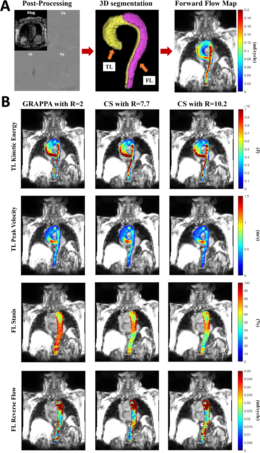
A) Represents postprocessing steps of the 4D Flow MRI data including processing of raw 4D Flow MR images on MATLAB and manual 3D segmentation of the true and false lumen B) True lumen peak velocity and kinetic energy and false lumen stasis and reverse flow maps in one subject with de novo type B aortic dissection and comparison of maps generated by MATLAB between conventional and compressed sensing accelerated 4D Flow MRI scans.
Parametric Hemodynamic Maps
3D parametric maps of aortic hemodynamics were derived using in-house analysis tools (MATLAB; The MathWorks, Natick, MA) similar to a recently reported workflow (6, 24). The 4D flow velocity data were interpolated to 1 mm3 voxels using spline interpolation. For each voxel KE, FF, 5th percentile PV, RF, and flow stasis were calculated inside the TL and FL in the patient group and in the entire aorta of the volunteers. A 3D aortic centerline was automatically calculated, and orthogonal analysis planes were automatically placed every millimeter along the center line. Each voxel was matched to the nearest plane to determine the direction of the flow from the normal vector, ie, forward (ascending aorta to descending aorta) and reverse (descending aorta to ascending aorta).
FF and RF:
Mean FF and RF were reported after summing the value in each voxel through the cardiac cycle, and then averaging these sums over the entire luminal volume.
KE:
Voxel-wise KE was defined by: KE = 0.5 × ρ × dV × v(t)2 where ρ is the assumed blood density of 1060 kg/m3, dV is the unit voxel volume (ie, 1 mm3) and v(t) is the velocity magnitude for each voxel at each cardiac time-frame. Total KE was reported by summing each voxel over the cardiac cycle.
PV:
The time point with the maximum 95th percentile voxel-wise PV was used to determine the 3D PV volumetric maps. The average of the maximum top 5% velocities was reported as PV for TL and FL.
Stasis:
Voxel-wise flow stasis was defined as the percentage of the cardiac timeframes in which the velocity in that voxel was < 0.1 m/s and this definition was used to generate volumetric stasis maps. Mean stasis was reported by averaging these percentages over the entire TL and FL volume.
Plane-based Flow Analysis
For time-resolved flow evaluation and average FF, RF and net flow (NF) quantifications, 2D planes were placed orthogonal to the at the TL both in the mid-ascending and mid-descending aorta and additionally to the midline of the FL in the descending aorta on the segmented volume of the aorta derived from each 4D Flow MRI scan (EnSight, version 211; CEI, Apex, NC, USA). The forward, retrograde and NFs were computed at each of these planes for all 4D Flow MRI acquisition types.
Statistical Analysis
Groupwise comparisons between acquisition types were performed using repeated measures analysis of variance (ANOVA) for voxelvise parameter values and plane-based flow quantifications. Pearson correlation coefficients (r) were also calculated for pairwise correlation of each voxelvise parameter in TL and FL among the acquisition types. Intraclass correlation coefficients (ICC) were calculated for interscan reliability assessment of each sequence type. ICC values less than 0.5 were indicative of poor reliability, between 0.5 and 0.75 moderate reliability, between 0.75 and 0.9 good reliability, and any value greater than 0.9 was indicative of excellent reliability (35). Average scan time and SD from the entire cohort consisting of both initial and repeat scans type were also reported for each acquisition type. For all analyses P < 0.05 was considered statistically significant.
RESULTS
Scan Times
Average scan time for conventional GRAPPA-accelerated 4D Flow MRI acquisition was 11.12 +/− 2.64 minutes whereas it was 5.13 +/− 1.80 minutes for CS7.7 and 4.01 +/− 1.23 minutes for CS10.2 acquisitions. The scan time reductions by CS-accelerated 4D Flow MRI acquisitions were 53.8% and 63.9% for CS7.7 and CS10.2 respectively when compared to the conventional 4D Flow MRI. The scan time reduction by CS7.7 was 21.8% when compared to CS10.2.
Hemodynamic 4D Flow MRI Parameters: True Lumen
The KE and FF in TL did not show significant differences among the three acquisition types (p = 0.818 and p = 0.065 respectively). The PV levels were significantly higher in GRAPPA compared to CS7.7 and CS10.2 acquisitions. The mean percent underestimations for PV were 4.76% and 6.34% for CS7.7 and CS10.2 acquisitions respectively. Mean RF was significantly lower in GRAPPA compared to CS10.2 with mean percent underestimation level of 6.25%. The mean stasis was significantly higher in GRAPPA compared to both CS7.7 and CS10.2 acquisitions with mean percent overestimation levels of 14.07% and 16.29% respectively. The Pearson correlation coefficients in the TL for all parameters in all pairwise comparisons among three acquisition types were as follows: r = 0.977, 0.951 and 0.980 for KE; 0.971, 0.943 and 0.960 for PV; 0.957, 0.961 and 0.986 for FF; 0.870, 0.781 and 0.902 for RF and lastly 0.810, 0.841 and 0.951 for stasis between GRAPPA and CS7.7, between GRAPPA and CS10.2 and between CS7.7 and CS10.2 acquisitions respectively. Mean and SDs of all parameters for all three acquisition types and Pearson correlation coefficients in the TL are summarized in table 3.
Table 3:
Summary of the mean and standard deviations of each true and false lumen parameter for each acquisition type, groupwise comparisons among three acquisition types and Pearson correlation coefficients.
| True Lumen | GRAPPA vs CS10.2 | GRAPPA vs CS7.7 | CS10.2 vs CS7.7 | False lumen | GRAPPA vs CS10.2 | GRAPPA vs CS7.7 | CS10.2 vs CS7.7 | ||||||||
|---|---|---|---|---|---|---|---|---|---|---|---|---|---|---|---|
| GRAPPA | CS10.2 | GRAPPA | CS7.7 | CS10.2 | CS7.7 | GRAPPA | CS10.2 | GRAPPA | CS7.7 | CS10.2 | CS7.7 | ||||
| Total Kinetic Energy (J) | Mean ± SD | 0.188 ± 0.079 | 0.184 ± 0.064 | 0.188 ± 0.079 | 0.186 ± 0.068 | 0.184 ± 0.064 | 0.186 ± 0.068 | Total Kinetic Energy (J) | Mean ± SD | 0.021 ± 0.013 | 0.038 ± 0.022 | 0.021 ± 0.013 | 0.035 ± 0019 | 0.038 ± 0.022 | 0.035 ± 0.019 |
| P value | 0.818 | P value | 0.008* | 0.003* | 0.374 | ||||||||||
| Correlation | 0.951* | 0.977* | 0.980* | Correlation | 0.733* | 0.861* | 0.928* | ||||||||
| %5 Peak Velocity (m/s) | Mean ± SD | 1.26 ± 0.26 | 1.18 ± 0.22 | 1.26 ± 026 | 1.20 ± 0.22 | 1.18 ± 0.22 | 1.20 ± 0.22 | %5 Peak Velocity (m/s) | Mean ± SD | 0.371 ± 0.148 | 0.441 ± 0.152 | 0.371 ± 0.148 | 0.408 ± 0.108 | 0.441 ± 0.152 | 0.408 ± 0.108 |
| P value | 0.002* | 0.006* | 0.627 | P value | 0.284 | ||||||||||
| (Correlation | 0.943* | 0.971* | 0.960* | Correlation | 0.455* | 0.879* | 0.738* | ||||||||
| Mean Forward Flow (ml/cycle) | Mean ± SD | 0.121 ± 0.030 | 0.121 ± 0.031 | 0.121 ± 0,030 | 0.125 ± 0.037 | 0.121 ± 0.031 | 0.125 ± 0.037 | Mean Forward Flow (ml/cycle) | Mean ± SD | 0.019 ± 0.008 | 0.024 ± 0.006 | 0.019 ± 0.008 | 0.024 ± 0,007 | 0.024 ± 0.006 | 0.024 ± 0.007 |
| P value | 0.065 | P value | 0.012* | 0.012* | 0.452 | ||||||||||
| Correlation | 0.961* | 0.957* | 0.986* | Correlation | 0.810* | 0.844* | 0.938* | ||||||||
| Mean Reverse Flow (ml/cycle) | Mean ± SD | 0.016 ± 0.005 | 0.017 ± 0.004 | 0.016 ± 0.005 | 0.017 ± 0.004 | 0.017 ± 0.004 | 0.017 ± 0.004 | Mean Reverse Flow (ml/cycle) | Mean ± SD | 0.016 ± 0.003 | 0.020 ± 0.003 | 0.016 ± 0.003 | 0.020 ± 0.003 | 0.020 ± 0.003 | 0.020 ± 0.003 |
| P value | 0.023* | 0.269 | 0.141 | P value | 0.023* | 0.010* | 0.986 | ||||||||
| Correlation | 0.781* | 0.870* | 0.902* | Correlation | 0.347 | 0.542* | 0.822* | ||||||||
| Mean Stasis (%) | Mean ± SD | 49.39 ± 7.92 | 41.34 ± 9.26 | 49.39 ± 7.92 | 42.44 ± 9.90 | 41.34 ± 9.26 | 42.44 ± 9.90 | Mean Stasis (%) | Mean ± SD | 80.13 ± 10.39 | 69.54 ± 11.60 | 80.13 ± 10.39 | 70.76 ± 10.69 | 69.54 ± 11.60 | 70.76 ± 10.69 |
| P value | 0.000* | 0.000* | 0.421 | P value | 0.003* | 0.001* | 0.500 | ||||||||
| Correlation | 0.841* | 0.810* | 0.951* | Correlation | 0.702* | 0798* | 0.948* | ||||||||
indicates statistical significance in repeated measures ANOVA and Pearson correlation coefficients
Hemodynamic 4D Flow MRI Parameters: False Lumen
The PV in the FL showed no significant difference among the three acquisition types (p = 0.284). In the FL, total KE, mean FF and mean RF values were significantly lower and mean stasis was significantly higher in GRAPPA compared to both the CS7.7 and the CS10.2 acquisitions. KE was the most sensitive parameter to CS imaging acceleration in FL with mean percent overestimations of 66.6% and 80.95% for CS7.7 and CS10.2 acquisitions respectively compared to GRAPPA 4D Flow MRI. There was overestimation of FF and RF in both CS acquisitions (26.3% and 25%, respectively), while stasis was underestimated by −11.6% with CS7.7 and −13.2% by CS10.2. There was no significant difference in FL KE, PV, FF, RF, and stasis between the two CS-accelerated acquisition (p = 0.374, 0.284, 0.452, 0.986 and 0.500, respectively).
Pearson correlation coefficients in the FL were as follows: r = 0.861, 0.879, 0.844, 0.542 and 0.798 for KE, PV, FF, RF and stasis respectively between GRAPPA and CS7.7 acquisitions; and r = 0.733, 0.455, 0.810, 0.702 for KE, PV, FF and stasis respectively between GRAPPA and CS10.2 acquisitions. No significant correlation was found for RF between GRAPPA and CS10.2 acquisitions (r = 0.347, p = 0.09). Pearson correlation coefficients between CS7.7 and CS10.2 acquisitions were 0.928, 0.738, 0.938, 0.822 and 0.948 for KE, PV, FF, RF and stasis respectively. Mean and SDs of all parameters for all three acquisition types and Pearson correlation coefficients in the FL are summarized in table 3. Boxplots for each parameter for the three acquisition types in TL and FL are shown in figure 2. Example descending aorta level cardiac coronal and sagittal images of all three acquisition types in one of the dnTBAD cases are shown in figure 3.
Figure 2:
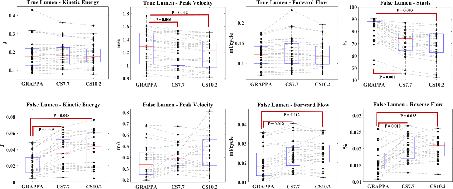
Boxplots represent the values for each parameter and the trend of their distribution among three acquisition types in true and false lumen. Statistically significant differences in pairwise comparisons are shown in the figure.
Figure 3:
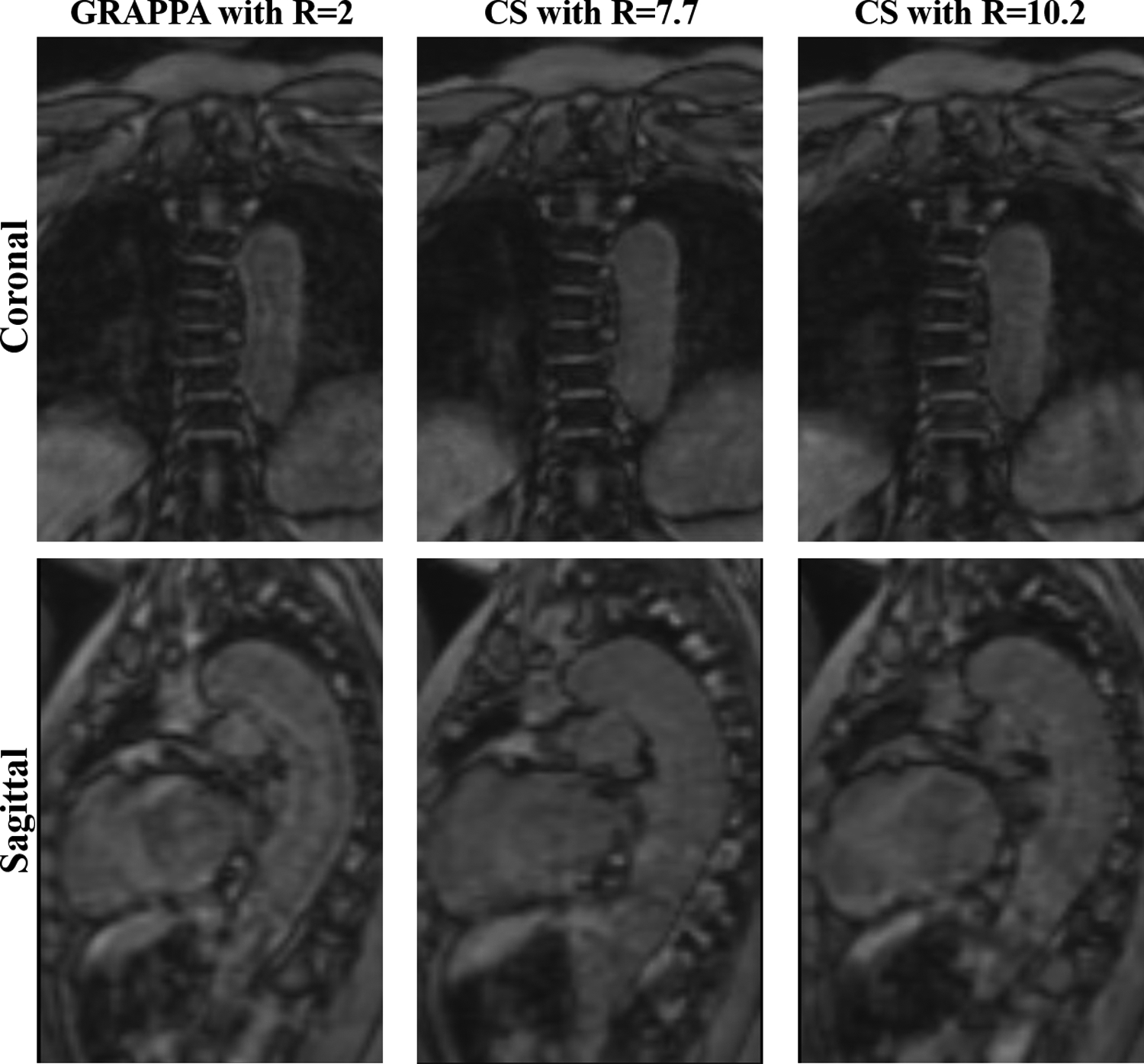
4D Flow MRI magnitude coronal and sagittal images for each acquisition type in one patient with de novo type B aortic dissection covering the lungs and thoracic descending aorta.
Plane-based Flow Analysis
Average FF values and their SDs in the TL were as follows: 73.76 +/− 20.98, 73.82 +/− 23.72 and 74.67 +/− 21.64 ml/cycle at the mid-ascending aorta level (p = 0.817) and 49.61 +/− 14.34, 46.80 +/− 14.14 and 46.33 +/− 15.49 ml/cycle at the mid-descending aorta level for GRAPPA, CS7.7 and CS10.2 acquisitions respectively. Mid-descending aorta TL FF were not significantly different between GRAPPA and CS7.7 acquisitions (p = 0.067) and between CS7.7 and CS10.2 acquisitions (p = 0.686). The FF analysis at the midline of the FL in the descending aorta showed the following results: 10.35 +/− 7.63, 10.07 +/− 7.51 and 10.24 +/− 7.64 ml/cycle (p = 0.796). Average RF values and their SDs in the TL were as follows: −2.16 +/− 2.87, −3.11 +/− 3.48 and −3.77 +/− 3.50 ml/cycle at mid-ascending aorta (p = 0.397) and −1.17 +/− 1.65, −1.47 +/− 2.34 and −1.50 +/− 2.40 ml/cycle at mid-descending aorta (p = 0.403) for GRAPPA, CS7.7 and CS10.2 acquisitions respectively. No significant result was observed in RF analysis in the mid-FL descending aorta analysis (−5.11 +/− 3.87, −5.09 +/− 5.21 and −5.29 +/− 4.14 ml/cycle for GRAPPA, CS7.7 and CS10.2 acquisitions respectively with a p value of 0.979). The last parameter in the plane-based flow quantifications was NF. Average NF values and their SDs in the TL were as follows: 70.63 +/− 19.39, 70.72 +/− 23.11 and 70.87 +/− 21.01 ml/cycle at the mid-ascending aorta (p = 0.992) and 48.44 +/− 14.31, 45.34 +/− 14.24 and 44.82 +/− 15.65 ml/cycle at the mid-descending aorta for GRAPPA, CS7.7 and CS10.2 acquisitions respectively. Comparisons between GRAPPA and CS7.7 acquisitions and between CS7.7 and CS10.2 acquisitions in the descending aorta were not significant (p = 0.069 and 0.689 respectively). And lastly NF analysis in the FL did not show significant difference among three acquisition types (5.23 +/− 6.73, 4.01 +/− 7.01 and 4.94 +/−7.43 ml/cycle for GRAPPA, CS7.7 and CS10.2 acquisitions respectively, p = 0.233).
Interscan Reliability Assessment
All TL parameters showed good to excellent reliability between initial and repeat scans for all three acquisition types in ICC analysis. The ICC levels for the TL between the first scan and second scans were 0.948, 0.957, 0.973, 0.936 and 0.955 for KE, PV, FF, RF and stasis respectively in GRAPPA 4D Flow MRI acquisition; 0.952, 0.956, 0.952, 0.909 and 0.856 respectively for CS7.7 acquisition and finally 0.937, 0.952, 0.966, 0.944 and 0.908 respectively for CS10.2 acquisition. A similar trend was observed for all five parameters in the FL. The ICCs for all five parameters including KE, stasis, PV, FF and RF between the first and second scans for GRAPPA-accelerated 4D Flow MRI were; 0.983, 0.974 0.989, 0.975 and 0.907 respectively. The ICCs for all five parameters between the first and second scans for CS7.7 acquisitions were 0.976, 0.973, 0.971, 0.925 and 0.884 respectively. Lastly, the ICC levels between the first and second scans for CS10.2 4D Flow MRI were 0.969, 0.958, 0.864 and 0.966 for KE, stasis, PV, FF respectively. The RF showed slightly lower, moderate level of agreement between the two scans for CS10.2 acquisition (r = 0.732). The ICCs between the first and second scans for each acquisition type are summarized in table 4.
Table 4:
Summary of intraclass correlation levels between the first and second scans 5–10 days apart for each acquisition type. All correlations showed statistical significance (p < 0.05)
| True Lumen | GRAPPA Scan 1 vs Scan 2 | CS7.7 Scan 1 vs Scan 2 | CS10.2 Scan 1 vs Scan 2 | |
|---|---|---|---|---|
| Intraclass Correlation Coefficients | Kinetic Energy (J) | 0.948 | 0.952 | 0.937 |
| Peak Velocity (m/s) | 0.957 | 0.956 | 0.952 | |
| Forward Flow (ml/cycle) | 0.973 | 0.952 | 0.966 | |
| Reverse Flow (ml/cycle) | 0.936 | 0.909 | 0.944 | |
| Stasis (%) | 0.955 | 0.856 | 0.908 | |
| False Lumen | GRAPPA Scan 1 vs Scan 2 | CS7.7 Scan 1 vs Scan 2 | CS10.2 Scan 1 vs Scan 2 | |
| Intraclass Correlation Coefficients | Kinetic Energy (J) | 0.983 | 0.976 | 0.969 |
| Peak Velocity (m/s) | 0.989 | 0.971 | 0.864 | |
| Forward Flow (ml/cycle) | 0.975 | 0.925 | 0.966 | |
| Reverse Flow (ml/cycle) | 0.907 | 0.884 | 0.732 | |
| Stasis (%) | 0.974 | 0.973 | 0.958 | |
DISCUSSION
Clinical implementation of 4D Flow MRI is hindered by long scan times even though its utility in evaluation of various cardiovascular pathologies has been widely supported (15–19). In this study we investigated the feasibility and performance of CS-accelerated 4D Flow MRI in TBAD cases with two different acceleration levels.
Despite the statistically significant difference between the TL PV and stasis values between conventional 4D Flow MRI and both CS-accelerated 4D Flow MRI acquisitions, and TL RF values between GRAPPA and CS10.2 acqusitions; these differences were small and within a clinically acceptable range. Additionally, stasis and RF are slow flow parameters and likely less clinically relevant in the TL compared to the FL.
On the other hand, FL results demonstrated overestimation of flow parameters (FF and RF) and KE, and underestimation of stasis values in both CS-accelerated acquisitions compared to traditional 4D Flow MRI. Among the hemodynamic parameters quantified, PV was the most stable parameter without any significant difference among the three acquisition types, while KE was the most sensitive parameter to CS imaging acceleration in FL. The KE value is obtained through a calculation directly proportional to velocity squared. In addition, CS acceleration tends to increase the noise in the images. Increased noisy voxels in CS reconstruction may be the driver of systematic overestimation and underestimation of these various parameters, particularly in the FL where signal and relative blood flows are both decreased, and the resultant velocity-to-noise ratio is already relatively low. Specifically for KE which is proportional to the velocity squared, any increase in noise introduced by the CS acceleration and quantified as a high velocity voxel will disproportionately impact KE more than other linear velocity or flow parameters. As Previous studies using CS based reconstruction methods have described underestimation of 4D Flow MRI derived flow parameters (19, 28–31). Pathrose et al evaluated the performance of CS-accelerated 4D Flow MRI at three acceleration factor levels (R = 5.7, 7.7, and 10.2) in a heterogenous cohort of patients with different aortic diseases including aortic root and ascending aortic dilation, bicuspid aortic valve, chronic TBAD and a patient with mechanical aortic valve replacement with ascending aortic aneurysm repair and demonstrated underestimation of several hemodynamic parameters by all CS protocols (19). However, their study included only four TBAD cases and they did not report the results specifically for the FL in the dissection cases. The plane-based mid-ascending and mid-descending TL and mid-FL flow analysis in our study showed statistically insignificant consistent values for almost all parameters among the three sequence types. The differences in TL FF and NF at the level of the mid-descending aorta between CS7.7 and CS10.2 are clinically negligible.
Neuhaus et al investigated the applicability of a six to eight-fold accelerated Cartesian CS aortic 4D Flow MRI technique with an inline reconstruction on the scanner (Compressed SENSE, Ingenia, Philips Healthcare). They showed no statistically significant differences in measured flow parameters (peak flow, NF and PV) between the reference SENSE-accelerated technique and the CS technique up to an acceleration rate of six (29). However, the R = 8 accelerated CS acquisition demonstrated underestimation of NF and a trend for underestimation of peak flow and statistically significant overestimation of PV when compared to the conventional SENSE-accelerated 4D Flow MRI acquisition. However, the CS technique used in their work combined the CS technique and the parallel imaging (SENSE) approaches and temporal correlations were not used in the reconstruction framework. In addition, their cohort did not include aortic dissection cases. The differences in the study population and image analysis might have contributed to the less significant differences between the conventional and CS-accelerated 4D Flow MRI approaches in their study compared to ours (29). Jarvis et al demonstrated the feasibility of hemodynamic mapping of conventional 4D Flow MRI as a quantitative technique for the characterization of chronic descending aortic dissection however they did not use CS-accelerated 4D Flow MRI (6). Chu et al used baseline 4D Flow MRI derived in vivo hemodynamic parameters to investigate their relationship with adverse aorta related outcomes in TBAD cases and demonstrated larger baseline diameters, lower RF and stasis in the FL and lower KE, FF and PV in the TL in patients with adverse aorta related outcomes in their overall cohort including both rTAAD and dnTBAD cases. Among patients with dnTBAD, patients with adverse aorta related outcomes had larger baseline diameter, lower FL stasis and TL PV. In both groups, subjects with aortic growth ≥ 3mm/year had a higher KE ratio. However, in that study traditional GRAPPA accelerated 4D Flow MRI was used and the impact of CS acceleration of 4D Flow MRI data was not investigated (24).
In our study, the scan times were reduced by 53.8% and 63.9% for CS-accelerated 4D Flow MRI scans with R = 7.7 and 10.2 respectively when compared to the conventional 4D Flow MRI. Three lines per segment were used for GRAPPA 4D Flow MRI acquisitions to reduce the acquisition time and 2 lines per segment were used for CS7.7 and CS10.2 acquisitions. These results may facilitate the clinical translation of CS-accelerated 4D Flow MRI as shorter scan times with increased imaging efficiency
The CS reconstruction techniques in our study were very similar to previously used techniques (19, 30). We have used them to perform hemodynamic quantifications and comprehensive evaluation of various flow parameters in TL and FL of TBAD. There are limited diagnostic or prognostic criteria for 4D Flow MRI derived hemodynamic parameters in TBAD, and a reference standard hemodynamic assessment for these patients is lacking. Considering these challenges, it is difficult to interpret the clinical importance of the differences seen in our study between CS-accelerated 4D Flow MRI acquisitions and conventional GRAPPA-accelerated 4D Flow MRI. However, given the scan time savings compared to conventional 4D Flow MRI, direct online reconstruction, and reliable results between initial and second scans with high interscan agreements, our results suggest the potential to integrate the CS-accelerated 4D Flow MRI in a clinical routine setting.
Limitations
The patient cohort in this study was small. Further work with larger populations may help evaluate hemodynamic features in TBAD with CS-accelerated 4D Flow MRI acquisitions and to establish reference normal ranges for each quantitative parameter with this technique. In addition, segmentation of aortic dissection remains challenging especially on non-contrast images and it may be improved by utilizing high blood-tissue contrast anatomical imaging registered to flow data or by exploring machine-learning algorithms to segment the FL. In addition, only one observer performed the segmentations. While this limitation may explain some of the variabilities in the values of the parameters among the acquisition types, our previous studies have showed excellent interobserver agreement (24). The order of the acquisition types was not systematically varied between subjects, which limits our ability to test for effects of time in scanner or acquisition order on hemodynamic differences. Using a static mask may have impacted the capture of the FL through the cardiac time point in cases where the FL was actively moving, and the velocity spectrum can be extremely large in TBAD patients which makes the choice of the VENC difficult. This could potentially be alleviated by using accelerated multi-VENC 4D Flow MRI acquisitions. Additionally, no other reconstruction parameters such as spatial and temporal regularizations and their effects on hemodynamic evaluations were explored in this study, and further work would be required to investigate these in TBAD cases. Additionally, the objective of this study was less about optimizing the CS acceleration performance and more about how currently available CS acceleration impacts advanced hemodynamic parameters in this unique cohort of patients. The main barriers currently to clinical implementation of the CS-accelerated 4D Flow MRI in TABD are: 1) an appreciation for impacts on hemodynamic quantification with CS acceleration which has been addressed in our study, and 2) availability of these acquisitions on clinical scanners.
Conclusion
Our study demonstrates that CS-accelerated 4D Flow MRI at acceleration factors of 7.7 and 10.2 had high agreement with conventional GRAPPA 4D Flow MRI in TL and overestimation of dynamic flow parameters in the FL in TBAD patients. Considering the unique patient population and the need to balance scan and reconstruction times, image quality, and accuracy of hemodynamic quantification, CS-accelerated 4D Flow MRI has the potential to become an integral aspect of hemodynamic evaluation in TBAD in the clinical settings.
Acknowledgements
The authors would like to thank Beth Whippo and Donny Nieto for their support in recruiting and scanning patients in this study.
Grant Support
Funding for this study was provided by the American Heart Association (20CDA35310687) and National Institutes of Health - National Institute of Biomedical Imaging & Bioengineering (T32EB025766).
REFERENCES
- 1.Zilber ZA, Boddu A, Malaisrie SC, et al. Noninvasive Morphologic and Hemodynamic Evaluation of Type B Aortic Dissection: State of the Art and Future Perspectives. Radiol Cardiothorac Imaging. 2021;3(3):e200456. [DOI] [PMC free article] [PubMed] [Google Scholar]
- 2.Malaisrie SC, Mehta CK. Updates on Indications for TEVAR in Type B Aortic Dissection. Innovations. 2020: 15(6):495–501 [DOI] [PubMed] [Google Scholar]
- 3.Malaisrie SC, Szeto WY, Halas M, et al. 2021 the American association for thoracic surgery expert consensus document: surgical treatment of acute type A aortic dissection. Journal Thorac Cardiovasc Surg. (2021) 162:735–758 [DOI] [PubMed] [Google Scholar]
- 4.Akin I, Nienaber CA. Prediction of aortic dissection. Heart. 2020;106(12):870–871. [DOI] [PubMed] [Google Scholar]
- 5.Elsayed RS, Cohen RG, Fleischman F, Bowdish ME. Acute Type A Aortic Dissection. Cardiology Clinics. 2017;35(3):331–345. [DOI] [PubMed] [Google Scholar]
- 6.Jarvis K, Pruijssen JT, Son AY, et al. Parametric Hemodynamic 4D Flow MRI Maps for the Characterization of Chronic Thoracic Descending Aortic Dissection. J Magn Reson Imaging. 2020;51(5):1357–1368. [DOI] [PMC free article] [PubMed] [Google Scholar]
- 7.Rohlffs F, Tsilimparis N, Diener H, et al. Chronic type B aortic dissection: indications and strategies for treatment. J Cardiovasc Surg (Torino). 2015;56(2):231–238. [PubMed] [Google Scholar]
- 8.Fattori R, Cao P, De Rango P, et al. Interdisciplinary expert consensus document on management of type B aortic dissection. J Am Coll Cardiol. 2013;61(16):1661–1678. [DOI] [PubMed] [Google Scholar]
- 9.Cooper M, Hicks C, Ratchford EV, Salameh MJ, Malas M. Diagnosis and treatment of uncomplicated type B aortic dissection. Vasc Med. 2016;21(6):547–552. [DOI] [PubMed] [Google Scholar]
- 10.van Bogerijen GH, Patel HJ, Williams DM, et al. Propensity adjusted analysis of open and endovascular thoracic aortic repair for chronic type B dissection: a twenty-year evaluation. Ann Thorac Surg. 2015;99(4):1260–1266. [DOI] [PubMed] [Google Scholar]
- 11.van Bogerijen GH, Tolenaar JL, Rampoldi V, et al. Predictors of aortic growth in uncomplicated type B aortic dissection. J Vasc Surg. 2014;59(4):1134–1143. [DOI] [PubMed] [Google Scholar]
- 12.Alfson DB, Ham SW. Type B Aortic Dissections: Current Guidelines for Treatment. Cardiol Clin. 2017;35(3):387–410. [DOI] [PubMed] [Google Scholar]
- 13.Usui A. TEVAR for type B aortic dissection in Japan. Gen Thorac Cardiovasc Surg. 2014;62(5):282–289. [DOI] [PubMed] [Google Scholar]
- 14.Borst HG, Walterbusch G, Schaps D. Extensive aortic replacement using “elephant trunk” prosthesis. Thorac Cardiovasc Surg. 1983;31(1):37–40. [DOI] [PubMed] [Google Scholar]
- 15.Burris NS, Hope MD. 4D flow MRI applications for aortic disease. Magn Reson Imaging Clin N Am. 2015;23(1):15–23. [DOI] [PMC free article] [PubMed] [Google Scholar]
- 16.Garcia J, Barker AJ, Markl M. The role of imaging of flow patterns by 4D flow MRI in aortic stenosis. JACC Cardiovasc Imaging. 2019;12(2):252–266. [DOI] [PubMed] [Google Scholar]
- 17.Hope MD, Meadows AK, Hope TA, et al. Clinical evaluation of aortic coarctation with 4D flow MR imaging. J Magn Reson Imaging. 2010;31(3):711–718. [DOI] [PubMed] [Google Scholar]
- 18.Bissell MM, Loudon M, Hess AT, et al. Differential flow improvements after valve replacements in bicuspid aortic valve disease: A cardiovascular magnetic resonance assessment. J Cardiovasc Magn Reson. 2018;20(1):10. [DOI] [PMC free article] [PubMed] [Google Scholar]
- 19.Pathrose A, Ma L, Berhane H, et al. Highly accelerated aortic 4D flow MRI using compressed sensing: Performance at different acceleration factors in patients with aortic disease. Magn Reson Med. 2021;85(4):2174–2187. [DOI] [PMC free article] [PubMed] [Google Scholar]
- 20.Marlevi D, Sotelo JA, Grogan-Kaylor R, et al. False lumen pressure estimation in type B aortic dissection using 4D flow cardiovascular magnetic resonance: comparisons with aortic growth. J Cardiovasc Magn Reson. 2021;23(1):51. [DOI] [PMC free article] [PubMed] [Google Scholar]
- 21.Burris NS, Nordsletten DA, Sotelo JA, et al. False lumen ejection fraction predicts growth in type B aortic dissection: preliminary results. Eur J Cardiothorac Surg. 2020;57(5):896–903. [DOI] [PMC free article] [PubMed] [Google Scholar]
- 22.Stankovic Z, Allen BD, Garcia J, Jarvis KB, Markl M. 4D flow imaging with MRI. Cardiovasc Diagn Ther. 2014;4(2):173–192. [DOI] [PMC free article] [PubMed] [Google Scholar]
- 23.Allen BD, Aouad PJ, Burris NS, et al. Detection and Hemodynamic Evaluation of Flap Fenestrations in Type B Aortic Dissection with 4D Flow MRI: Comparison with Conventional MRI and CTA. Radiol Cardiothorac Imaging. 2019;1(1):e180009. [DOI] [PMC free article] [PubMed] [Google Scholar]
- 24.Chu S, Kilinc O, Pradella M, et al. Baseline 4D Flow-Derived in vivo Hemodynamic Parameters Stratify Descending Aortic Dissection Patients With Enlarging Aortas. Front. Cardiovasc. Med 2022;9:905718. [DOI] [PMC free article] [PubMed] [Google Scholar]
- 25.Clough RE, Waltham M, Giese D, Taylor PR, Schaeffter T. A new imaging method for assessment of aortic dissection using four-dimensional phase contrast magnetic resonance imaging. J Vasc Surg. 2012;55(4):914–923. [DOI] [PubMed] [Google Scholar]
- 26.Basha TA, Akçakaya M, Goddu B, Berg S, Nezafat R. Accelerated three-dimensional cine phase contrast imaging using randomly undersampled echo planar imaging with compressed sensing reconstruction. NMR Biomed. 2015;28(1):30–39. [DOI] [PubMed] [Google Scholar]
- 27.Cheng JY, Hanneman K, Zhang T, et al. Comprehensive motion-compensated highly accelerated 4D flow MRI with ferumoxytol enhancement for pediatric congenital heart disease. J Magn Reson Imaging. 2016;43(6):1355–1368. [DOI] [PMC free article] [PubMed] [Google Scholar]
- 28.Dyvorne H, Knight-Greenfield A, Jajamovich G, et al. Abdominal 4D flow MR imaging in a breath hold: Combination of spiral sampling and dynamic compressed sensing for highly accelerated acquisition. Radiology. 2015;275(1):245–254. [DOI] [PMC free article] [PubMed] [Google Scholar]
- 29.Neuhaus E, Weiss K, Bastkowski R, Koopmann J, Maintz D, Giese D. Accelerated aortic 4D flow cardiovascular magnetic resonance using compressed sensing: applicability, validation and clinical integration. J Cardiovasc Magn Reson. 2019;21(1):65. [DOI] [PMC free article] [PubMed] [Google Scholar]
- 30.Ma LE, Markl M, Chow K, et al. Aortic 4D flow MRI in 2 minutes using compressed sensing, respiratory controlled adaptive k-space reordering, and inline reconstruction. Magn Reson Med. 2019;81(6):3675–3690. [DOI] [PMC free article] [PubMed] [Google Scholar]
- 31.Hsiao A, Lustig M, Alley MT, Murphy MJ, Vasanawala SS. Evaluation of valvular insufficiency and shunts with parallel-imaging compressed-sensing 4D phase-contrast MR imaging with stereoscopic 3D velocity-fusion volume-rendered visualization. Radiology. 2012;265(1):87–95. [DOI] [PMC free article] [PubMed] [Google Scholar]
- 32.Gottwald LM, Peper ES, Zhang Q, et al. Pseudo-spiral sampling and compressed sensing reconstruction provides flexibility of temporal resolution in accelerated aortic 4D flow MRI: A comparison with k-t principal component analysis. NMR Biomed. 2020;33(4):e4255. [DOI] [PMC free article] [PubMed] [Google Scholar]
- 33.Bernstein MA, Zhou XJ, Polzin JA, et al. Concomitant gradient terms in phase contrast MR: analysis and correction. Magn Reson Med. 1998;39(2):300–308. [DOI] [PubMed] [Google Scholar]
- 34.Walker PG, Cranney GB, Scheidegger MB, Waseleski G, Pohost GM, Yoganathan AP. Semiautomated method for noise reduction and background phase error correction in MR phase velocity data. J Magn Reson Imaging. 1993;3(3):521–530. [DOI] [PubMed] [Google Scholar]
- 35.Bobak CA, Barr PJ, O’Malley AJ. Estimation of an inter-rater intra-class correlation coefficient that overcomes common assumption violations in the assessment of health measurement scales. BMC Med Res Methodol. 2018;12;18(1):93. [DOI] [PMC free article] [PubMed] [Google Scholar]