Stochastic analysis of a COVID-19 model with effects of vaccination and different transition rates: Real data approach

Abstract

This paper presents a stochastic model for COVID-19 that takes into account factors such as incubation times, vaccine effectiveness, and quarantine periods in the spread of the virus in symptomatically contagious populations. The paper outlines the conditions necessary for the existence and uniqueness of a global solution for the stochastic model. Additionally, the paper employs nonlinear analysis to demonstrate some results on the ergodic aspect of the stochastic model. The model is also simulated and compared to deterministic dynamics. To validate and demonstrate the usefulness of the proposed system, the paper compares the results of the infected class with actual cases from Iraq, Bangladesh, and Croatia. Furthermore, the paper visualizes the impact of vaccination rates and transition rates on the dynamics of infected people in the infected class.

1. Introduction

COVID-19, caused by the severe acute respiratory syndrome coronavirus 2 (SARS-CoV-2), is a respiratory illness that is highly infectious. It was first identified in Wuhan, China in December 2019 and has quickly spread across the globe, resulting in a pandemic.

The symptoms of COVID-19 range from moderate to severe ones and can include fever, cough, shortness of breath, body aches, fatigue, loss of taste or smell, and a sore throat. Some people may have only mild symptoms or no symptoms at all, but others can develop severe respiratory problems that can cause hospitalization and death, especially in older individuals and people having previous unhealthy conditions.

The transmission of the COVID-19 virus is primarily through respiratory droplets, which are released when an infected person coughs, talks, or sneezes. In addition, it is also possible to contract the virus by touching a surface contaminated with the virus and then touching one’s face.

To prevent the spread of COVID-19, it is important to practice better hygiene, such as frequently washing hands regularly, wearing a mask in public settings, and maintaining social distance from others. Vaccines have also been developed and authorized for emergency use, which can help to reduce the infection’s risk and also severity of symptoms.

Governments and health organizations around the world are working together to contain the spread of COVID-19 and to provide care and support to those who have been affected. The response to the pandemic has included measures such as lockdowns, travel restrictions, and widespread testing and contact tracing.

The COVID-19 outbreak has had a significant and far-reaching effect on the globe, affecting the health and well-being of individuals, the global economy, and societies at large. The response to the pandemic continues to evolve as more is learned about the virus and the development of effective treatments and vaccines. We list some mathematical models of COVID-19 in [1], [2], [3], [4], [5].

Recently, a team of researchers led by Yavuz [6] created a mathematical model to study the spread of COVID-19 among symptomatically contagious populations. The model takes into consideration the impact of factors such as incubation time, vaccine efficacy, and quarantine measures. The population of is divided into six categories for the purpose of the model. The first category, denoted by $\mathbf{S}$, consists of susceptible individuals who are not yet infected with the virus. The second category, denoted by $\mathbf{E}$, consists of exposed individuals who have come in contact with the virus but do not display symptoms and can spread the virus to others. The third category, denoted by $\mathbf{I}$, consists of infected individuals who have contracted the virus. The fourth category, denoted by $\mathbf{Q}$, includes individuals who have been quarantined to prevent further spread of the virus, with the quarantine period equal to the longest incubation time of COVID-19. The fifth category, denoted by $\mathbf{V}$, includes post-vaccinated individuals. Finally, the sixth category, denoted by $\mathbf{R}$, consists of recovered individuals who have acquired immunity against COVID-19. However, some of these individuals may still be susceptible to the virus in the future.

$$\frac{d\mathbf{S}}{dt}=\mathcal{A}+\zeta \mathbf{V}-\mathbf{S}\left(\frac{\delta \mathbf{E}}{\mathbf{N}}+k_1+\nu \right),$$

$$\frac{d\mathbf{E}}{dt}=\mathbf{E}\left(\frac{\delta \mathbf{S}}{\mathbf{N}}-{\beta }_1-{\omega }_1-\nu \right),$$

$$\frac{d\mathbf{I}}{dt}={\beta }_1\mathbf{E}-\mathbf{I}\left({\vartheta }_1+{\omega }_2+\nu +{\nu }_1\right),$$ (1)

$$\frac{d\mathbf{Q}}{dt}={\omega }_1\mathbf{E}+{\omega }_2\mathbf{I}-\mathbf{Q}\left({\vartheta }_2+\nu \right),$$

$$\frac{d\mathbf{V}}{dt}=k_1\mathbf{S}-\mathbf{V}\left(\zeta +\nu \right),$$

$$\frac{d\mathbf{R}}{dt}={\vartheta }_1\mathbf{I}+{\vartheta }_2\mathbf{Q}-\nu \mathbf{R},$$

subject to

$$\left\{\begin{array}{c}{\mathbf{S}}_0={\mathbf{S}}_0\ge 0,{\mathbf{E}}_0={\mathbf{E}}_0\ge 0,{\mathbf{I}}_0={\mathbf{I}}_0\ge 0,{\mathbf{Q}}_0={\mathbf{Q}}_0\ge 0,\hfill \\ {\mathbf{V}}_0={\mathbf{V}}_0\ge 0,{\mathbf{R}}_0={\mathbf{R}}_0\ge 0,\hfill \end{array}\right)$$

where the total population $\mathbf{N}=\mathbf{S}+\mathbf{E}+\mathbf{I}+\mathbf{Q}+\mathbf{V}+\mathbf{R}$.

Stochastic differential equations (SDEs) are mathematical models that describe the evolution of a system over time in the presence of randomness or uncertainty. They are used in a wide range of applications, including finance, physics, biology, and engineering, among others [7], [8], [9].

SDEs are a generalization of ordinary differential equations (ODEs), which describe the evolution of a deterministic system over time. The difference is that in SDEs, the evolution of the system is affected by random disturbances, represented by a stochastic process.

In finance, SDEs are used to model the evolution of stock prices, interest rates, and other financial variables. In physics, they are used to model the motion of particles in random media, such as Brownian motion. In biology, they are used to model the spread of diseases, genetic evolution, and other biological processes. In engineering, they are used to model the behavior of systems with random disturbances, such as power grids and communication networks. SDEs have been used to analyze epidemic mathematical models over the last few years. Sazonov et al. investigated stochastic HIV model based on Markov Chain [10]. Frei et al. proposed a cancer metastasis using SDEs [11]. Also, SDEs were used for modeling of COVID-19 pandemic. Adak et al. investigated dynamical behavior of stochastic COVID-19 model [12]. The authors in [13] studied COVID-19 for a case study in Pakistan using SDEs. Some more works on stochastic models of COVID-19 can be found in [14], [15], [16].

In stochastic form the model (1) can be written as,

$$d\mathbf{S}\left(t\right)=\left[\mathcal{A}+\zeta \mathbf{V}-\mathbf{S}\left(\frac{\delta \mathbf{E}}{\mathbf{N}}+k_1+\nu \right)\right]dt+{\varsigma }_1\mathbf{S}\left(t\right)d{\mathfrak{M}}_1\left(t\right),$$

$$d\mathbf{E}\left(t\right)=\left[\mathbf{E}\left(\frac{\delta \mathbf{S}}{\mathbf{N}}-{\beta }_1-{\omega }_1-\nu \right)\right]dt+{\varsigma }_2\mathbf{E}\left(t\right)d{\mathfrak{M}}_2\left(t\right),$$

$$d\mathbf{I}\left(t\right)=\left[{\beta }_1\mathbf{E}-\mathbf{I}\left(\vartheta +{\omega }_2+\nu +{\nu }_1\right)\right]dt+{\varsigma }_3\mathbf{I}\left(t\right)d{\mathfrak{M}}_3\left(t\right),$$ (2)

$$d\mathbf{Q}\left(t\right)=\left[{\omega }_1\mathbf{E}+{\omega }_2\mathbf{I}-\mathbf{Q}\left({\vartheta }_2+\nu \right)\right]dt+{\varsigma }_4\mathbf{Q}\left(t\right)d{\mathfrak{M}}_4\left(t\right),$$

$$d\mathbf{V}\left(t\right)=\left[k_1\mathbf{S}-\mathbf{V}\left(\zeta +\nu \right)\right]dt+{\varsigma }_5\mathbf{V}\left(t\right)d{\mathfrak{M}}_5\left(t\right),$$

$$d\mathbf{R}\left(t\right)=\left[{\vartheta }_1\mathbf{I}+{\vartheta }_2\mathbf{Q}-\nu \mathbf{R}\right]dt+{\varsigma }_6\mathbf{R}\left(t\right)d{\mathfrak{M}}_6\left(t\right).$$

In the above model ${\mathfrak{M}}_i\left(t\right)$ and ${\varsigma }_i$ stands for Brownian motion and intensities of noise for $(i=1,2,\dots ,6)$ are the noise intensities. In this paper, suppose $(\Theta ,\Pi ,{\left(\Pi \right)}_{0\le t,Z})$ is a space of complete probability where ${{\Pi }_t}_0$ satisfy the condition i.e it is increasing and right continuous where ${\Pi }_0$ consist of Z null-sets, further ${\mathfrak{M}}_i\left(t\right)$ is specified on the entire probabilities’ space. We use the notations as: ${\mathbb{R}}_{+}^y=(x_1,\dots ,x_y):0<x_y,y\ge i\ge 1,\mathrm{a}\vee \mathrm{b}=max\{\mathrm{a},\mathrm{b}\},\mathrm{a}\wedge \mathrm{b}=min\{\mathrm{a},\mathrm{b}\}$, and $〈\mathrm{U}〉={\int }_0^t\mathrm{U}\left(r\right)dr$.

2. Mathematical analysis of the model (2)

Here, we study and analyze the stochastic COVID-19 model (2). Let $\mathrm{Y}\left(t\right)$ be a Markov process in ${\mathcal{R}}^d$ that is both regular and time-homogeneous. This process can be described by a stochastic differential equation as

$$d\mathrm{Y}\left(t\right)=\mathrm{U}\left(\mathrm{Y}\left(t\right)\right)dt+h\left(\mathrm{Y}\left(t\right)\right)d\mathfrak{M}\left(t\right).$$ (3)

We define matrix of diffusion as $\mathrm{A}=\left({\mathrm{a}}_{ij}\left(x\right)\right),{\mathrm{a}}_{ij}\left(x\right)=h^i\left(x\right)h^j\left(x\right)$, where the operator of diffusion $\mathcal{L}$ is given by,

$$\mathcal{L}=\sum _{i=1}^d{h}_i\left(x\right)\frac{\partial }{\partial x_i}+\sum _{i,j=1}^d{\mathrm{a}}_{ij}\left(x\right)\frac{{\partial }^2}{\partial x_i\partial x_j}.$$ (4)

If the operator $\mathcal{L}$ is applied on function $\mathcal{A}\in {\mathcal{C}}^2({\mathcal{R}}^d,{\mathcal{R}}_{+})$, then

$$\mathcal{L}\mathcal{A}\left(x\right)={\mathcal{A}}_x\left(x\right)\mathrm{U}\left(x\right)+\frac{1}{2}trace\left[h^T\left(x\right){\mathcal{A}}_{xx}h\left(x\right)\right],$$ (5)

here

$${\mathcal{A}}_x\left(x\right)=\left(\frac{\partial \mathcal{A}}{\partial x_i},\dots ,\frac{\partial \mathcal{A}}{\partial x_d}\right),{\mathcal{A}}_{xx}=\frac{{\partial }^2\mathcal{A}}{\partial x_i\partial x_j}.$$ (6)

2.1. Existence, uniqueness of solution

Here, we present results for positivity and uniqueness of the solution of model (2).

Theorem 2.1

For each initial value $({\mathbf{S}}_0,{\mathbf{E}}_0,{\mathbf{I}}_0,{\mathbf{Q}}_0,{\mathbf{V}}_0,{\mathbf{R}}_0)\in {\mathcal{R}}_{+}^6$ , there exists non-negative solution $(\mathbf{S}\left(t\right),\mathbf{E}\left(t\right),\mathbf{I}\left(t\right),\mathbf{Q}\left(t\right),\mathbf{V}\left(t\right),\mathbf{R}\left(t\right))$ of model (2) on $0\le \mathrm{t}$ and also stay in ${\mathcal{R}}_{+}^6$ having probability 1.

Proof

As we know that the coefficient of model (2) satisfy Lipschitz condition, so the initial value $({\mathbf{S}}_0,{\mathbf{E}}_0,{\mathbf{I}}_0,{\mathbf{Q}}_0,{\mathbf{V}}_0,{\mathbf{R}}_0)\in {\mathcal{R}}_{+}^6$, and there exists a non-negative solution $(\mathbf{S}\left(t\right),\mathbf{E}\left(t\right),\mathbf{I}\left(t\right),\mathbf{Q}\left(t\right),\mathbf{V}\left(t\right),\mathbf{R}\left(t\right))$ of model (2) for $\mathrm{t}\in [0,{\mathfrak{A}}_e)$, here ${\mathfrak{A}}_e$ is time of explosion see [30]. Now we have to show that the solution of (2) is global, for this, we need to show that ${\mathfrak{A}}_e=\infty$. To take start, suppose $k_0$ is a non negative real number sufficiently large i.e all the initial values lies in the interval $[\frac{1}{k_0},k]$, we define stopping time for $k\ge k_0$:

$${\mathfrak{A}}_k=\left\{t\in [0,{\mathfrak{A}}_e):min\left(\left(\mathbf{S}\left(t\right),\mathbf{E}\left(t\right),\mathbf{I}\left(t\right),\mathbf{Q}\left(t\right),\mathbf{V}\left(t\right),\mathbf{R}\left(t\right)\right)\right\}\le \frac{1}{k}\right\}ork\ge max\left\{\left(\mathbf{S}\left(t\right),\mathbf{E}\left(t\right),\mathbf{I}\left(t\right),\mathbf{Q}\left(t\right),\mathbf{V}\left(t\right),\mathbf{R}\left(t\right)\right)\right\}.$$ (7)

Further, we assume that $inf(\varnothing )=\infty$, ($\varnothing$ describe empty set). We say that ${\mathfrak{A}}_k$ is of increasing type when $k\to \infty$. Suppose ${lim}_{k\to \infty }{\mathfrak{A}}_k={\mathfrak{A}}_{\infty }$. If for all $t\in [0,\infty )$, we need to show ${\mathfrak{A}}_{\infty }=\infty$. It can also be written as ${\mathfrak{A}}_e=\infty$ and $\left(\mathbf{S}\left(t\right),\mathbf{E}\left(t\right),\mathbf{I}\left(t\right),\mathbf{Q}\left(t\right),\mathbf{V}\left(t\right),\mathbf{R}\left(t\right)\right)\in {\mathcal{R}}_{+}^6$. If our assumption is not true, then $\exists$ constant $\mathcal{F}>0$ and $ϵ\in (0,1)$ such that

$$P\{{\mathfrak{A}}_{\infty }\le \mathcal{F}\}>ϵ.$$ (8)

Now, we consider $\mathcal{H}:{\mathcal{R}}_{+}^6\to {\mathcal{R}}_{+}$, which is taken from $C^2$ space and is defined as

$$\begin{array}{cc}\mathcal{H}\left(\mathbf{S},\mathbf{E},\mathbf{I},\mathbf{Q},\mathbf{V},\mathbf{R}\right)=\hfill & \mathcal{L}\mathcal{H}\left(\mathbf{S},\mathbf{E},\mathbf{I},\mathbf{Q},\mathbf{V},\mathbf{R}\right)dt\hfill \\ \hfill & -5-\left(log\mathbf{S}+log\mathbf{E}+log\mathbf{I}+log\mathbf{Q}+log\mathbf{V}+log\mathbf{R}\right).\hfill \end{array}$$

Now we apply the basics for all $y>0$, $-1+y-logy\ge$, we express $\mathcal{H}\ge 0$. Now let $k\ge k_0$ and $\mathcal{F}\ge {\mathcal{F}}_0$, by applying Ito results on Eq. (9), we obtain

$$\mathrm{d}\mathcal{H}\left(\mathbf{S},\mathbf{E},\mathbf{I},\mathbf{Q},\mathbf{V},\mathbf{R}\right)=\mathcal{L}\mathcal{H}\left(\mathbf{S},\mathbf{E},\mathbf{I},\mathbf{Q},\mathbf{V},\mathbf{R}\right)dt+{\varsigma }_1(\mathbf{S}-1)d{\mathfrak{M}}_1\left(t\right)+{\varsigma }_2(\mathbf{E}-1)\mathrm{d}{\mathfrak{M}}_2\left(t\right)$$ (9)

$$+{\varsigma }_3(\mathbf{I}-1)\mathrm{d}{\mathfrak{M}}_3\left(t\right)+{\varsigma }_4(\mathbf{Q}-1)\mathrm{d}{\mathfrak{M}}_4\left(t\right)+{\varsigma }_5(\mathbf{V}-1)d{\mathfrak{M}}_5\left(t\right)+{\varsigma }_6(\mathbf{R}-1)\mathrm{d}{\mathfrak{M}}_6\left(t\right).$$

In the above equation, $\mathcal{L}\mathcal{H}:{\mathcal{R}}_{+}^6\to {\mathcal{R}}_{+}$ is presented by

$$\mathcal{L}\mathcal{H}\left(\mathbf{S},\mathbf{E},\mathbf{I},\mathbf{Q},\mathbf{V},\mathbf{R}\right)=\left(1-\frac{1}{\mathbf{S}}\right)\left(\mathcal{A}+\zeta \mathbf{V}-\mathbf{S}\left(\frac{\delta \mathbf{E}}{\mathbf{N}}+k_1+\nu \right)\right)$$ (10)

$$+\left(1-\frac{1}{\mathbf{E}}\right)\left(\mathbf{E}\left(\frac{\delta \mathbf{S}}{\mathbf{N}}-{\beta }_1-{\omega }_1-\nu \right)\right)+\left(1-\frac{1}{\mathbf{I}}\right)\left({\beta }_1\mathbf{E}-\mathbf{I}\left(\vartheta +{\omega }_2+\nu +{\nu }_1\right)\right)+\left(1-\frac{1}{\mathbf{Q}}\right)\left({\omega }_1\mathbf{E}+{\omega }_2\mathbf{I}-\mathbf{Q}\left({\vartheta }_2+\nu \right)\right)+\left(1-\frac{1}{\mathbf{V}}\right)\left(k_1\mathbf{S}-\mathbf{V}\left(\zeta +\nu \right)\right)+\left(1-\frac{1}{\mathbf{R}}\right)\left({\vartheta }_1\mathbf{I}+{\vartheta }_2\mathbf{Q}-\nu \mathbf{R}\right)+\frac{{ϵ}_1^2+{ϵ}_2^2+{ϵ}_3^2+{ϵ}_4^2+{ϵ}_5^2+{ϵ}_6^2}{2}=\mathcal{A}+\zeta \mathbf{V}-\mathbf{S}\left(\frac{\delta \mathbf{E}}{\mathbf{N}}+k_1+\nu \right)-\frac{\mathcal{A}}{\mathbf{S}}-\frac{\zeta \mathbf{V}}{\mathbf{S}}+\left(\frac{\delta \mathbf{E}}{\mathbf{N}}+k_1+\nu \right)+\frac{{ϵ}_1^2}{2}+\mathbf{E}\left(\frac{\delta \mathbf{S}}{\mathbf{N}}-{\beta }_1-{\omega }_1-\nu \right)+\mathbf{E}\left(\frac{\delta \mathbf{S}}{\mathbf{N}}+{\beta }_1+{\omega }_1+\nu \right)+\frac{{ϵ}_2^2}{2}+{\beta }_1\mathbf{E}-\mathbf{I}\left(\vartheta +{\omega }_2+\nu +{\nu }_1\right)-\frac{{\beta }_1\mathbf{E}}{\mathbf{I}}+\left(\vartheta +{\omega }_2+\nu +{\nu }_1\right)+\frac{{ϵ}_3^2}{2}+{\omega }_1\mathbf{E}+{\omega }_2\mathbf{I}-\mathbf{Q}\left({\vartheta }_2+\nu \right)-\frac{{\omega }_1\mathbf{E}}{\mathbf{Q}}-\frac{{\omega }_2\mathbf{I}}{\mathbf{Q}}+\left({\vartheta }_2+\nu \right)+\frac{{ϵ}_4^2}{2}$$ (11)

$$+k_1\mathbf{S}-\mathbf{V}\left(\zeta +\nu \right)-\frac{k_1\mathbf{S}}{\mathbf{V}}+\left(\zeta +\nu \right)+\frac{{ϵ}_5^2}{2}+{\vartheta }_1\mathbf{I}+{\vartheta }_2\mathbf{Q}-\nu \mathbf{R}-\frac{{\vartheta }_1\mathbf{I}}{\mathbf{R}}-\frac{{\vartheta }_2\mathbf{Q}}{\mathbf{R}}+\nu +\frac{{ϵ}_6^2}{2}\le \mathcal{A}+(k_1+\nu )+\left(\vartheta +{\omega }_2+\nu +{\nu }_1\right)+\left({\vartheta }_2+\nu \right)+\left(\zeta +\nu \right)+\nu +\frac{{ϵ}_1^2+{ϵ}_2^2+{ϵ}_3^2+{ϵ}_4^2+{ϵ}_5^2+{ϵ}_6^2}{2}$$ (12)

$$\le \mathcal{A}+k_1+5\nu +\vartheta +{\vartheta }_2+{\omega }_2+{\nu }_1+\zeta +\frac{{ϵ}_1^2+{ϵ}_2^2+{ϵ}_3^2+{ϵ}_4^2+{ϵ}_5^2+{ϵ}_6^2}{2}=\mathcal{K}.$$

In the above equation $\mathcal{K}$ is non negative, it has no independent and state variable. Thus

$$\mathrm{d}\mathcal{H}\left(\mathbf{S},\mathbf{E},\mathbf{I},\mathbf{Q},\mathbf{V},\mathbf{R}\right)=\mathcal{K}dt+{\varsigma }_1(\mathbf{S}-1)\mathrm{d}{\mathfrak{M}}_1\left(t\right)+{\varsigma }_2(\mathbf{E}-1)\mathrm{d}{\mathfrak{M}}_2\left(t\right)$$ (13)

$$+{\varsigma }_3(\mathbf{I}-1)\mathrm{d}{\mathfrak{M}}_3\left(t\right)+{\varsigma }_4(\mathbf{Q}-1)\mathrm{d}{\mathfrak{M}}_4\left(t\right)+{\varsigma }_5(\mathbf{V}-1)d{\mathfrak{M}}_5\left(t\right)+{\varsigma }_6(\mathbf{R}-1)\mathrm{d}{\mathfrak{M}}_6\left(t\right).$$

Furthermore, we integrate Eq. (13), so we obtain

$$\mathbb{E}[\mathbf{S}({\mathfrak{A}}_k\wedge \mathcal{F}),\mathbf{E}({\mathfrak{A}}_k\wedge \mathcal{F}),\mathbf{I}({\mathfrak{A}}_k\wedge \mathcal{F}),\mathbf{Q}({\mathfrak{A}}_k\wedge \mathcal{F}),\mathbf{V}({\mathfrak{A}}_k\wedge \mathcal{F}),\mathbf{R}({\mathfrak{A}}_k\wedge \mathcal{F})]$$ (14)

$$\le \mathcal{H}({\mathbf{S}}_0,{\mathbf{E}}_0,{\mathbf{I}}_0,{\mathbf{Q}}_0,{\mathbf{V}}_0,{\mathbf{R}}_0)+\mathbf{E}\left[{\int }_0^{{\mathfrak{A}}_k\wedge \mathcal{F}}\mathcal{K}\right]$$

$$\le \mathcal{H}({\mathbf{S}}_0,{\mathbf{E}}_0,{\mathbf{I}}_0,{\mathbf{Q}}_0,{\mathbf{V}}_0,{\mathbf{R}}_0)+\mathcal{F}\mathcal{K}.$$

Taking ${\Phi }_k=\{\varpi \in \Phi :\mathcal{F}\ge {\mathfrak{A}}_k\left(\varpi \right)={\mathfrak{A}}_k\}$ for $k\ge k_1$ and Eq. (8) become, $P\left({\Phi }_k\right)\ge ϵ$. Here we observe that for all $\varpi$ one or more then one $\mathbf{S}({\mathfrak{A}}_k,\varpi ),\mathbf{E}({\mathfrak{A}}_k,\varpi ),\mathbf{I}({\mathfrak{A}}_k,\varpi ),\mathbf{Q}({\mathfrak{A}}_k,\varpi ),\mathbf{V}({\mathfrak{A}}_k,\varpi ),\mathbf{R}({\mathfrak{A}}_k,\varpi )$ which is equal to $k$ or $\frac{1}{k}$. So

$$\mathcal{H}(\mathbf{S}({\mathfrak{A}}_k,\varpi ),\mathbf{E}({\mathfrak{A}}_k,\varpi ),\mathbf{I}({\mathfrak{A}}_k,\varpi ),\mathbf{Q}({\mathfrak{A}}_k,\varpi ),\mathbf{V}({\mathfrak{A}}_k,\varpi ),\mathbf{R}({\mathfrak{A}}_k,\varpi ))\ge (\frac{1}{k}-1-log\left(\frac{1}{k}\right))\wedge (k-1-logk).$$ (15)

From Eqs. (14), (15), one can obtain

$$\mathcal{H}({\mathbf{S}}_0,{\mathbf{E}}_0,{\mathbf{I}}_0,{\mathbf{Q}}_0,{\mathbf{V}}_0,{\mathbf{R}}_0)+\mathcal{F}\mathcal{K}\ge \mathbf{E}\left(I_{\Phi k\left(\varpi \right)}\mathcal{H}(\mathbf{S}({\mathfrak{A}}_k,\varpi ),\mathbf{E}({\mathfrak{A}}_k,\varpi ),\mathbf{I}({\mathfrak{A}}_k,\varpi ),\mathbf{Q}({\mathfrak{A}}_k,\varpi ),\mathbf{V}({\mathfrak{A}}_k,\varpi ),\mathbf{R}({\mathfrak{A}}_k,\varpi ))\right)\ge ϵ[(k-logk-1)\wedge (\frac{1}{k}-log\left(\frac{1}{k}\right)-1)],$$ (16)

here $I_{\Phi k\left(\varpi \right)}$ is a function of $\Phi \left(t\right)$ i.e indicator function. Suppose $k\to \infty$, then

$$\infty >\mathcal{H}({\mathbf{S}}_0,{\mathbf{E}}_0,{\mathbf{I}}_0,{\mathbf{Q}}_0,{\mathbf{V}}_0,{\mathbf{R}}_0)+\mathcal{F}\mathcal{K}=\infty ,$$ (17)

this is a contradiction. Hence we conclude that ${\mathfrak{A}}_k=\infty$. This completes the proof.

3. Extinction of the model

To model the dynamical aspects of our proposed model (2), we investigate when the disease tend to extinct. In this section we show that the stochastic model (2) vanishes. Suppose

$$\mathfrak{M}\left(\mathrm{t}\right)=\frac{1}{\mathrm{t}}{\int }_0^{\mathrm{t}}\mathfrak{M}\left(s\right)ds.$$ (18)

Lemma 3.1

Let us take $\left(\mathbf{S}\mathbf{E}\mathbf{I}\mathbf{Q}\mathbf{V}\mathbf{R}\right)$ is solution of model (1) with initial condition $\left(\mathbf{S}\mathbf{E}\mathbf{I}\mathbf{Q}\mathbf{V}\mathbf{R}\right)\in {\mathcal{R}}_{+}^6$ , so

$$\underset{\mathrm{t}\to \infty }{lim}\frac{\left(\mathbf{S}\left(\mathrm{t}\right)+\mathbf{I}\left(\mathrm{t}\right)+\mathbf{E}\left(\mathrm{t}\right)+\mathbf{Q}\left(\mathrm{t}\right)+\mathbf{R}\left(\mathrm{t}\right)+\mathbf{V}\left(\mathrm{t}\right)\right)}{\mathrm{t}}=0.$$ (19)

Further if ${\nu }_0>\frac{{\varsigma }_1^2\vee {\varsigma }_2^2\vee {\varsigma }_3^2\vee {\varsigma }_4^2\vee {\varsigma }_5^2\vee {\varsigma }_6^2}{2}$ then

$$\underset{\mathrm{t}\to \infty }{lim}\frac{1}{\mathrm{t}}{\int }_0^{\mathrm{t}}\mathbf{S}\left(\mathrm{u}\right)d{\mathfrak{M}}_1\left(\mathrm{u}\right)=0,\underset{\mathrm{t}\to \infty }{lim}\frac{1}{\mathrm{t}}{\int }_0^{\mathrm{t}}\mathbf{E}\left(\mathrm{u}\right)d{\mathfrak{M}}_2\left(\mathrm{u}\right)=0,\underset{\mathrm{t}\to \infty }{lim}\frac{1}{\mathrm{t}}{\int }_0^{\mathrm{t}}\mathbf{I}\left(\mathrm{u}\right)d{\mathfrak{M}}_3\left(\mathrm{u}\right)=0,\underset{\mathrm{t}\to \infty }{lim}\frac{1}{\mathrm{t}}{\int }_0^{\mathrm{t}}\mathbf{Q}\left(\mathrm{u}\right)d{\mathfrak{M}}_4\left(\mathrm{u}\right)=0,\underset{\mathrm{t}\to \infty }{lim}\frac{1}{\mathrm{t}}{\int }_0^{\mathrm{t}}\mathbf{V}\left(\mathrm{u}\right)d{\mathfrak{M}}_5\left(\mathrm{u}\right)=0.\underset{\mathrm{t}\to \infty }{lim}\frac{1}{\mathrm{t}}{\int }_0^{\mathrm{t}}\mathbf{R}\left(\mathrm{u}\right)d{\mathfrak{M}}_6\left(\mathrm{u}\right)=0.$$

This lemma can be proved by simple calculation. For our proposed model, we prove the theorem presented below.

Theorem 3.1

Let $(\mathbf{S}\left(t\right),\mathbf{E}\left(t\right),\mathbf{I}\left(t\right),\mathbf{Q}\left(t\right),\mathbf{V}\left(t\right),\mathbf{R}\left(t\right))$ be solution of model (2) with initial condition $({\mathbf{S}}_0,{\mathbf{E}}_0,{\mathbf{I}}_0,{\mathbf{Q}}_0,{\mathbf{V}}_0,{\mathbf{R}}_0)\in R^5$ . Further, if ${\mu }_0>\frac{{ϵ}_1^2+{ϵ}_2^2+{ϵ}_3^2+{ϵ}_4^2+{ϵ}_5^2+{ϵ}_6^2}{2}$ and $1>R_0$ .

$$\underset{t\to \infty }{lim}\frac{〈log\mathbf{E}\left(t\right)〉}{t}<0,and\underset{t\to \infty }{lim}\frac{〈log\mathbf{I}\left(t\right)〉}{t}<0,$$ (20)

here, $\mathbf{E}\left(t\right)$ as it is sure that the disease eliminate with probability one as it goes to zero exponentially. Moreover,

$$\underset{t\to \infty }{lim}〈\mathbf{S}\left(t\right)〉=\frac{A(\zeta +\nu )-k_1}{\nu (\zeta +\nu )},\underset{t\to \infty }{lim}〈\mathbf{E}\left(t\right)〉=0,\underset{t\to \infty }{lim}〈\mathbf{I}\left(t\right)〉=0,$$ (21)

$$\underset{t\to \infty }{lim}〈\mathbf{Q}\left(t\right)〉=0,\underset{t\to \infty }{lim}〈\mathbf{V}\left(t\right)〉=\frac{k1A}{\nu (\zeta +\nu )},\underset{t\to \infty }{lim}〈\mathbf{R}\left(t\right)〉=0.$$

Proof

Using integration on model (2), we have

$$\frac{1}{t}(\mathbf{S}\left(t\right)-{\mathbf{S}}_0)=\mathcal{A}+\zeta \mathbf{V}-\mathbf{S}\left(\frac{\delta \mathbf{E}}{\mathbf{N}}+k_1+\nu \right)+\frac{{\varsigma }_1}{t}{\int }_0^t\mathbf{S}\left(r\right)d{\mathfrak{M}}_1\left(r\right)$$

$$\frac{1}{t}(\mathbf{E}\left(t\right)-{\mathbf{E}}_0)=\mathbf{E}\left(\frac{\delta \mathbf{S}}{\mathbf{N}}-{\beta }_1-{\omega }_1-\nu \right)+\frac{{\varsigma }_2}{t}{\int }_0^t\mathbf{E}\left(r\right)d{\mathfrak{M}}_2\left(r\right)$$

$$\frac{1}{t}(\mathbf{I}\left(t\right)-{\mathbf{I}}_0)={\beta }_1\mathbf{E}-\mathbf{I}\left(\vartheta +{\omega }_2+\nu +{\nu }_1\right)+\frac{{\varsigma }_3}{t}{\int }_0^t\mathbf{I}\left(r\right)d{\mathfrak{M}}_3\left(r\right)$$ (22)

$$\frac{1}{t}(\mathbf{Q}\left(t\right)-{\mathbf{Q}}_0)={\omega }_1\mathbf{E}+{\omega }_2\mathbf{I}-\mathbf{Q}\left({\vartheta }_2+\nu \right)+\frac{{\varsigma }_4}{t}{\int }_0^t\mathbf{Q}\left(r\right)d{\mathfrak{M}}_4\left(r\right)$$

$$\frac{1}{t}(\mathbf{V}\left(t\right)-{\mathbf{V}}_0)=k_1\mathbf{S}-\mathbf{V}\left(\zeta +\nu \right)+\frac{{\varsigma }_5}{t}{\int }_0^t\mathbf{V}\left(r\right)d{\mathfrak{M}}_5\left(r\right)$$

$$\frac{1}{t}(\mathbf{R}\left(t\right)-{\mathbf{R}}_0)={\vartheta }_1\mathbf{I}+{\vartheta }_2\mathbf{Q}-\nu \mathbf{R}+\frac{{\varsigma }_6}{t}{\int }_0^t\mathbf{R}\left(r\right)d{\mathfrak{M}}_6\left(r\right).$$

Using Ito formula on the second equation of model (2) will be in the form,

$$dlog\mathbf{E}\left(t\right)=\left[\mathbf{E}\left(\frac{\delta \mathbf{S}}{\mathbf{N}}-{\beta }_1-{\omega }_1-\nu \right)-\frac{{\varsigma }_2^2}{2}\right]dt+{\varsigma }_{2}d{\mathfrak{M}}_2\left(r\right).$$ (23)

Further we integrate Eq. (23) from 0 to t, we get

$$\frac{log\mathbf{E}\left(t\right)-log{\mathbf{E}}_0}{t}=\left(\frac{\delta \mathbf{S}}{\mathbf{N}}-{\beta }_1-{\omega }_1-\nu \right)-\frac{{\varsigma }_2^2}{2}+\frac{{\varsigma }_2}{t}{\int }_0^{t}d{\mathfrak{M}}_2\left(r\right)\le \delta -\left({\beta }_1+{\omega }_1+\nu +\frac{{\varsigma }_2^2}{2}\right)+\frac{{\varsigma }_2}{t}{\int }_0^{t}d{\mathfrak{M}}_2\left(r\right)=\delta -\left({\beta }_1+{\omega }_1+\nu +\frac{{\varsigma }_2^2}{2}\right)+\frac{{\varsigma }_2}{t}{\int }_0^{t}d{\mathfrak{M}}_2\left(r\right)=\left({\beta }_1+{\omega }_1+\nu +\frac{{\varsigma }_2^2}{2}\right)(R_0-1)+\frac{{\varsigma }_2}{t}{\int }_0^{t}d{\mathfrak{M}}_2\left(r\right).$$ (24)

However, $\mathcal{M}\left(t\right)=\frac{{\varsigma }_2}{t}{\int }_0^{t}d{\mathfrak{M}}_2\left(r\right)$, and $\mathcal{M}\left(t\right)$ is local continuous (martingale) and ${\mathcal{M}}_0=0$. Further from the Lemma 3.1, and if $t\to \infty$, we get

$$\underset{t\to \infty }{lim}sup\frac{\mathcal{M}\left(t\right)}{t}=0.$$ (25)

If the condition i.e $R_0<1$ is verified, then Eq. (24) becomes

$$\underset{t\to \infty }{lim}sup\frac{log\mathbf{E}}{t}\le \left({\beta }_1+{\omega }_1+\nu +\frac{{\varsigma }_2^2}{2}\right)(R_0-1)<0.$$ (26)

From Eq. (26) we obtain,

$$\underset{t\to \infty }{lim}\mathbf{E}\left(t\right)=0.$$ (27)

Furthermore, the 3rd equation of model (2) with integrating having limit from 0 to t and obtain equation is divided by t, we get

$$\frac{\mathbf{I}\left(t\right)-{\mathbf{I}}_0}{t}={\beta }_1\mathbf{E}-\mathbf{I}\left(\vartheta +{\omega }_2+\nu +{\nu }_1\right)+\frac{{\varsigma }_3}{t}{\int }_0^t\mathbf{I}\left(r\right)d{\mathfrak{M}}_3\left(r\right)$$ (28)

$$〈\mathbf{I}\left(t\right)〉=\frac{1}{\vartheta +{\omega }_2+\nu +{\nu }_1}\left[{\beta }_1\mathbf{E}+\frac{{\mathbf{I}}_0-\mathbf{I}\left(t\right)}{t}+\frac{{\varsigma }_3}{t}{\int }_0^t\mathbf{I}\left(r\right)d{\mathfrak{M}}_3\left(r\right)\right].$$ (29)

Thus

$$\underset{t\to \infty }{lim}\mathbf{I}\left(t\right)=0.$$ (30)

The fourth and sixth equation of (22), and using Eqs. (31), (30), and $t\to \infty$, then we get

$$\underset{t\to \infty }{lim}\mathbf{Q}\left(t\right)=0,\underset{t\to \infty }{lim}\mathbf{R}\left(t\right)=0.$$ (31)

From Eq. (22), we obtain

$$\frac{\mathbf{S}\left(t\right)-{\mathbf{S}}_0+\mathbf{V}\left(t\right)-{\mathbf{V}}_0}{t}=A+\zeta \mathbf{V}-\frac{\mathbf{S}\delta \mathbf{E}}{\mathbf{N}}-\mathbf{S}{k}_1+\mathbf{S}\nu +\frac{{\varsigma }_1}{t}{\int }_0^t\mathbf{S}\left(r\right)\mathfrak{M}\left(r\right)+k_1\mathbf{S}\zeta \mathbf{V}-\nu \mathbf{V}+\frac{{\varsigma }_5}{t}{\int }_0^t\mathbf{V}\left(r\right)\mathfrak{M}\left(r\right)$$ (32)

$$〈\mathbf{S}\left(t\right)+\mathbf{V}\left(t\right)〉=\frac{A}{\nu }+\Phi \left(t\right),$$

here $\Phi \left(t\right)$ is,

$$\Phi \left(t\right)=-\frac{1}{\nu }\left[\frac{1}{t}(\mathbf{S}\left(t\right)-{\mathbf{S}}_0)+\frac{1}{t}(\mathbf{V}\left(t\right)-{\mathbf{V}}_0)\right)\left(-\frac{{\varsigma }_1}{t}{\int }_0^t\mathbf{S}\left(r\right)d{\mathfrak{M}}_1\left(r\right)-\frac{{\varsigma }_5}{t}{\int }_0^t\mathbf{V}\left(r\right)d{\mathfrak{M}}_5\left(r\right)\right].$$ (33)

As $t\to \infty$ then definitely $\Phi \left(t\right)\to 0$, so we obtain

$$\nu 〈\mathbf{S}\left(t\right)〉+\nu 〈\mathbf{V}\left(t\right)〉=A.$$ (34)

From Eq. (22), we have

$$\frac{\mathbf{V}\left(t\right)-{\mathbf{V}}_0}{t}=k_1\mathbf{S}-\nu (\nu +\zeta )+\frac{{\varsigma }_5}{t}{\int }_0^t\mathbf{V}\left(r\right)d{\mathfrak{M}}_5\left(r\right)$$

$$k_1\mathbf{S}-\nu (\nu +\zeta )=-\frac{1}{t}(\mathbf{V}\left(t\right)-{\mathbf{V}}_0)-\frac{{\varsigma }_5}{t}{\int }_0^t\mathbf{V}\left(r\right)d{\mathfrak{M}}_5\left(r\right).$$ (35)

If $t\to \infty$ in Eq. (35), then we get

$$k_1\mathbf{S}-\nu (\zeta +\nu )=0.$$ (36)

From Eqs. (34) and (36), we obtain

$$\underset{t\to \infty }{lim}〈\mathbf{S}\left(t\right)〉=\frac{A[(\zeta +\nu )-k_1]}{\nu (\zeta +\nu )},$$ (37)

$$\underset{t\to \infty }{lim}〈\mathbf{V}\left(t\right)〉=\frac{k_{1}A}{\nu (\zeta +\nu )},$$ (38)

which is the required proof. □

Lemma 3.2

If an open domain $\mathcal{D}$ is present within ${\mathcal{E}}_d$ , and its boundary ${\rm Y}$ is of a regular type with characteristic, then process of Markov $\mathcal{X}\left(\mathcal{F}\right)$ will possess unique ergodic distribution of stationary nature denoted by $\Omega \left(\cdot \right)$ .

$\mathbf{a}$ . For each $ħ\in {\mathcal{E}}_d$ , the matrix $\mathcal{G}$ should be positive-definite.

$\mathbf{b}$ . For $ħ\in {\mathcal{E}}_d\setminus \mathcal{D}$ , $\mathcal{F}$ is finite mean-time which is the required time from $ħ$ to $\mathcal{D}$ , and ${sup}_{ħ\in \mathcal{K}}{\mathcal{E}}_d\setminus \mathcal{D}<\infty$ for $\mathcal{K}\in {\mathcal{E}}_d$ , are the whole compact subsets. So

$${\mathcal{P}}_{ħ}\left\{\underset{\mathcal{F}\to \infty }{lim}\frac{1}{T\mathcal{F}}{\int }_0^{\mathcal{F}}f\left(\mathcal{X}\right)d\mathcal{F}={\int }_{{\mathcal{E}}_d}f(ħ)\Omega (dħ)\right\},forallħ\in \mathcal{E}=1.$$ (39)

where $f(.)$ is the function describe the integrability of $f$ with respect to $\Omega$ .

Theorem 3.2

Let

$${\mathcal{R}}_0^s=\frac{\nu \delta }{\left(k_1+\nu +\frac{{\varsigma }_1^2}{2}\right)\left({\beta }_1+{\omega }_1+\nu +\frac{{\varsigma }_2^2}{2}\right)}.$$ (40)

The model (2) have only stationary distribution $\Omega (.)$ , which have characteristic of ergodicity.

Proof

From Theorem 2.1, we conclude that for initial values $\left({\mathbf{S}}_0,{\mathbf{E}}_0,{\mathbf{I}}_0,{\mathbf{Q}}_0,{\mathbf{V}}_0,{\mathbf{R}}_0\right)\in {\mathcal{R}}^6$, $\exists$ unique and non-local solutions of $\left(\mathbf{S},\mathbf{E},\mathbf{I},\mathbf{Q},\mathbf{V},\mathbf{R}\right)\in {\mathcal{R}}^6$. Furthermore, the t diffusion equation for our proposed model (2) can be written as,

$$\mathfrak{M}=\left(\begin{array}{cccccc}\hfill {\varsigma }_1^2{\mathbf{S}}^2\hfill & \hfill 0\hfill & \hfill 0\hfill & \hfill 0\hfill & \hfill 0\hfill & \hfill 0\hfill \\ \hfill 0\hfill & \hfill {\varsigma }_2^2{\mathbf{E}}^2\hfill & \hfill 0\hfill & \hfill 0\hfill & \hfill 0\hfill & \hfill 0\hfill \\ \hfill 0\hfill & \hfill 0\hfill & \hfill {\varsigma }_3^2{\mathbf{I}}^2\hfill & \hfill 0\hfill & \hfill 0\hfill & \hfill 0\hfill \\ \hfill 0\hfill & \hfill 0\hfill & \hfill 0\hfill & \hfill {\varsigma }_4^2{\mathbf{Q}}^2\hfill & \hfill 0\hfill & \hfill 0\hfill \\ \hfill 0\hfill & \hfill 0\hfill & \hfill 0\hfill & \hfill 0\hfill & \hfill {\varsigma }_5^2{\mathbf{V}}^2\hfill & \hfill 0\hfill \\ \hfill 0\hfill & \hfill 0\hfill & \hfill 0\hfill & \hfill 0\hfill & \hfill 0\hfill & \hfill {\varsigma }_6^2{\mathbf{R}}^2\hfill \\ \hfill \left(\mathbf{S}\mathbf{E}\mathbf{I}\mathbf{Q}\mathbf{V}\mathbf{R}\right)\in {\mathcal{R}}^6\hfill & \hfill \hfill & \hfill \hfill & \hfill \hfill & \hfill \hfill & \hfill \hfill \end{array}\right).$$ (41)

Now take $\mathcal{M}={min}_{\left(\mathbf{S},\mathbf{E},\mathbf{I},\mathbf{Q},\mathbf{V},\mathbf{R}\right)\in {\mathcal{R}}^6}\{{\varsigma }_1^2{\mathbf{S}}^2,{\varsigma }_2^2{\mathbf{E}}^2,{\varsigma }_3^2{\mathbf{I}}^2,{\varsigma }_4^2{\mathbf{Q}}^2,{\varsigma }_5^2{\mathbf{V}}^2,{\varsigma }_6^2{\mathbf{R}}^2\}$, we get

$$\sum _{i,j=1}^4{\mathrm{a}}_{\mathrm{ij}}\left(\mathbf{S},\mathbf{E},\mathbf{I},\mathbf{Q},\mathbf{V},\mathbf{R}\right){\eta }_i{\eta }_j={\varsigma }_1^2{\mathbf{S}}^2{\eta }_1^2+{\varsigma }_2^2{\mathbf{E}}^2{\eta }_2^2+{\varsigma }_3^2{\mathbf{I}}^2{\eta }_3^2+{\varsigma }_4^2{\mathbf{Q}}^2{\eta }_4^2$$ (42)

$$+{\varsigma }_5^2{\mathbf{V}}^2{\eta }_5^2+{\varsigma }_6^2{\mathbf{R}}^2{\eta }_6^2\ge \mathcal{M}\mid \eta {\mid }^2,\left(Z,R,X,Y\right)\in \mathcal{D},$$

where $\eta =\left({\eta }_1,{\eta }_2,{\eta }_3,{\eta }_4,{\eta }_5,{\eta }_6\right)\in {\mathcal{R}}_{+}^6$. Then condition (a) of 2nd lemma is satisfied. Furthermore, we consider $\mathcal{H}:{\mathcal{R}}_{+}^4\to {\mathcal{R}}_{+}$ in the present theorem. Here our prime focus is the proving of part (b) of 2nd lemma. To prove this we consider a positive ${\mathcal{C}}^2$ function $\mathcal{H}:{\mathcal{R}}_{+}^6\to {\mathcal{R}}_{+}$. First we define,

$${\mathcal{H}}_1=\mathbf{S}+\mathbf{I}+\mathbf{E}\mathbf{Q}+\mathbf{V}+\mathbf{R}-{\mathcal{U}}_{1}ln\left(\mathbf{S}\right)-{\mathcal{U}}_{2}ln\left(\mathbf{E}\right)-{\mathcal{U}}_{3}ln\left(\mathbf{I}\right),$$ (43)

where ${\mathcal{U}}_1$, ${\mathcal{U}}_2$, ${\mathcal{U}}_3$ are positive constants which are to be found later. Using Ito’s formula in light of model (2), we obtain

$$\mathcal{L}\left(\mathbf{S}+\mathbf{I}+\mathbf{E}+\mathbf{Q}+\mathbf{V}+\mathbf{R}\right)=A-\nu \left(\mathbf{S}+\mathbf{I}+\mathbf{E}+\mathbf{Q}+\mathbf{V}+\mathbf{R}\right)-{\nu }_1\mathbf{I},$$

$$\mathcal{L}(-ln\left(\mathbf{S}\right))=-\frac{A}{\mathbf{S}}-\frac{\xi \mathbf{V}}{\mathbf{S}}+\left(\frac{\delta \mathbf{E}}{N}-k_1+\nu \right)+\frac{{\varsigma }_1}{t}$$

$$\mathcal{L}(-ln\left(\mathbf{E}\right))=-\left(\frac{\delta \mathbf{E}}{N}-{\beta }_1-{\omega }_1-\nu \right)+\frac{{\varsigma }_2}{t}$$

$$\mathcal{L}(-ln\left(\mathbf{I}\right))=-\frac{{\beta }_1\mathbf{E}}{\mathbf{I}}+(\vartheta +{\omega }_2+\nu +{\nu }_1)+\frac{{\varsigma }_3}{t}$$ (44)

$$\mathcal{L}(-ln\left(\mathbf{Q}\right))=-\frac{{\omega }_1\mathbf{E}}{\mathbf{V}}-\frac{{\omega }_2\mathbf{I}}{\mathbf{V}}+({\vartheta }_2+\nu )+\frac{{\varsigma }_4}{t}$$

$$\mathcal{L}(-ln\mathbf{V})=-\frac{k_1\mathbf{S}}{\mathbf{V}}+(\xi +\nu )+\frac{{\varsigma }_5}{t}$$

$$\mathcal{L}(-ln\left(\mathbf{R}\right))=-\frac{{\vartheta }_1\mathbf{I}}{\mathbf{R}}-\frac{{\vartheta }_2\mathbf{Q}}{\mathbf{R}}+\nu +\frac{{\varsigma }_6}{t},$$

so we have

$$\mathcal{L}{\mathcal{H}}_1=A-\nu \left(\mathbf{S}+\mathbf{I}+\mathbf{E}+\mathbf{Q}+\mathbf{V}+\mathbf{R}\right)-{\nu }_1\mathbf{I}+{\mathcal{U}}_1\left(-\frac{A}{\mathbf{S}}-\frac{\xi \mathbf{V}}{\mathbf{S}}+\left(\frac{\delta \mathbf{E}}{N}-k_1+\nu \right)+\frac{{\varsigma }_1}{t}\right)+{\mathcal{U}}_2\left(-\left(\frac{\delta \mathbf{E}}{N}-{\beta }_1-{\omega }_1-\nu \right)+\frac{{\varsigma }_2}{t}\right)+{\mathcal{U}}_3\left(-\frac{{\beta }_1\mathbf{E}}{\mathbf{I}}+(\vartheta +{\omega }_2+\nu +{\nu }_1)+\frac{{\varsigma }_3}{t}\right)=A-\nu \left(\mathbf{S}+\mathbf{I}+\mathbf{E}+\mathbf{Q}+\mathbf{R}+\mathbf{V}\right)-{\nu }_1\mathbf{I}+-{\mathcal{U}}_1\frac{A}{\mathbf{S}}-{\mathcal{U}}_1\frac{\xi \mathbf{V}}{\mathbf{S}}+{\mathcal{U}}_1\frac{\delta \mathbf{E}}{N}-{\mathcal{U}}_1{k}_1+{\mathcal{U}}_1\nu +{\mathcal{U}}_1\frac{{\varsigma }_1}{t}-{\mathcal{U}}_2\frac{\delta \mathbf{E}}{N}+{\mathcal{U}}_2{\beta }_1+{\mathcal{U}}_2{\omega }_1+{\mathcal{U}}_2\nu +{\mathcal{U}}_2\frac{{\varsigma }_2}{t}+{\mathcal{U}}_3-{\mathcal{U}}_3\frac{{\beta }_1\mathbf{E}}{\mathbf{I}}+{\mathcal{U}}_3(\vartheta +{\omega }_2+\nu +{\nu }_1)+{\mathcal{U}}_3\frac{{\varsigma }_3}{t}\le -3{\left[\nu \left(\mathbf{S}+\mathbf{E}+\mathbf{I}+\mathbf{Q}+\mathbf{V}+\mathbf{R}\right)\frac{{\mathcal{U}}_{1}A}{\mathbf{S}}\frac{{\mathcal{U}}_2\delta \mathbf{E}}{N}\right]}^{\frac{1}{3}}+A+{\mathcal{U}}_1\left(k_1+\nu +\frac{{\varsigma }_1^2}{2}\right)+{\mathcal{U}}_2\left({\beta }_1+{\omega }_1+\nu +\frac{{\varsigma }_2^2}{2}\right)+{\mathcal{U}}_3\left(\vartheta +{\omega }_2+\nu +{\nu }_1+\frac{{\varsigma }_3^2}{2}\right)-\nu \mathbf{I}-{\mathcal{U}}_1\frac{\xi \mathbf{V}}{\mathbf{S}}+{\mathcal{U}}_1\frac{\delta \mathbf{E}}{N}-{\mathcal{U}}_3\frac{{\beta }_1\mathbf{E}}{\mathbf{I}}.$$ (45)

From Eq. (45), we have

$$\mathcal{L}{\mathcal{H}}_1\le -3{\left({\mathcal{U}}_1{\mathcal{U}}_2\nu \delta A\right)}^{\frac{1}{3}}+A+{\mathcal{U}}_1\left(k_1+\nu +\frac{{\varsigma }_1^2}{2}\right)+{\mathcal{U}}_2\left({\beta }_1+{\omega }_1+\nu +\frac{{\varsigma }_2^2}{2}\right)$$ (46)

$$+{\mathcal{U}}_3\left(\vartheta +{\omega }_2+\nu +{\nu }_1+\frac{{\varsigma }_3^2}{2}\right)-\nu \mathbf{I}-{\mathcal{U}}_1\frac{\xi \mathbf{V}}{\mathbf{S}}+{\mathcal{U}}_1\frac{\delta \mathbf{E}}{N}-{\mathcal{U}}_3\frac{{\beta }_1\mathbf{E}}{\mathbf{I}}.$$

Suppose

$$A={\mathcal{U}}_1\left(k_1+\nu +\frac{{\varsigma }_1^2}{2}\right)={\mathcal{U}}_2\left({\beta }_1+{\omega }_1+\nu +\frac{{\varsigma }_2^2}{2}\right)={\mathcal{U}}_3\left(\vartheta +{\omega }_2+\nu +{\nu }_1+\frac{{\varsigma }_3^2}{2}\right),$$ (47)

where

$${\mathcal{U}}_1=\frac{A}{\left(k_1+\nu +\frac{{\varsigma }_1^2}{2}\right)},$$

$${\mathcal{U}}_2=\frac{A}{\left({\beta }_1+{\omega }_1+\nu +\frac{{\varsigma }_2^2}{2}\right)},$$

$${\mathcal{U}}_3=\frac{A}{\left(\vartheta +{\omega }_2+\nu +{\nu }_1+\frac{{\varsigma }_3^2}{2}\right)}.$$ (48)

Therefore

$$\mathcal{L}{\mathcal{H}}_1\le -3{\left[\left(\frac{\nu \delta {\left(A\right)}^3}{\left(k_1+\nu +\frac{{\varsigma }_1^2}{2}\right)\left({\beta }_1+{\omega }_1+\nu +\frac{{\varsigma }_2^2}{2}\right)}\right)-A\right]}^{\frac{1}{3}}+{\mathcal{U}}_3\left(\vartheta +{\omega }_2+\nu +{\nu }_1+\frac{{\varsigma }_3^2}{2}\right)-\nu \mathbf{I}-{\mathcal{U}}_1\frac{\xi \mathbf{V}}{\mathbf{S}}+{\mathcal{U}}_1\frac{\delta \mathbf{E}}{N}-{\mathcal{U}}_3\frac{{\beta }_1\mathbf{E}}{\mathbf{I}}$$ (49)

$$\mathcal{L}{\mathcal{H}}_1\le -3A\left[{\left({\mathcal{R}}_0^s\right)}^{\frac{1}{3}}-1\right]+{\mathcal{U}}_3\left(\vartheta +{\omega }_2+\nu +{\nu }_1+\frac{{\varsigma }_3^2}{2}\right)-\nu \mathbf{I}-{\mathcal{U}}_1\frac{\xi \mathbf{V}}{\mathbf{S}}+{\mathcal{U}}_1\frac{\delta \mathbf{E}}{N}-{\mathcal{U}}_3\frac{{\beta }_1\mathbf{E}}{\mathbf{I}}.$$ (50)

Furthermore, we get

$${\mathcal{H}}_2={\mathcal{U}}_4\left(\mathbf{S}+\mathbf{I}+\mathbf{E}+\mathbf{Q}+\mathbf{V}+\mathbf{R}-{\mathcal{U}}_{1}ln\left(\mathbf{S}\right)-{\mathcal{U}}_{2}ln\left(\mathbf{E}\right)-{\mathcal{U}}_{3}ln\left(\mathbf{I}\right)\right)-ln\left(\mathbf{S}\right)-ln\left(\mathbf{Q}\right)-ln\left(\mathbf{V}\right)-ln\left(\mathbf{R}\right)+\mathbf{S}+\mathbf{I}+\mathbf{E}+\mathbf{Q}+\mathbf{V}+\mathbf{R}=({\mathcal{U}}_4+1)\left(\mathbf{S}+\mathbf{E}+\mathbf{I}+\mathbf{Q}+\mathbf{V}+\mathbf{R}\right)-({\mathcal{U}}_4{\mathcal{U}}_1+1)ln\mathbf{S}-{\mathcal{U}}_2{\mathcal{U}}_{4}ln\mathbf{E}-{\mathcal{U}}_3{\mathcal{U}}_{4}ln\mathbf{I}-ln\mathbf{Q}-ln\mathbf{V}-ln\mathbf{R},$$ (51)

where ${\mathcal{U}}_4>0$ is a constant to be calculate later. We define

$$lim\underset{\left(\mathbf{S},\mathbf{E},\mathbf{I},\mathbf{Q},\mathbf{V},\mathbf{R}\right)\in \underset{+}{\overset{6}{\mathcal{R}}}}{inf}\setminus {\mathcal{G}}_k{\mathcal{H}}_2\left(\mathbf{S},\mathbf{E},\mathbf{I},\mathbf{Q},\mathbf{V},\mathbf{R}\right)=+\infty ,\text{as}k\to \infty ,$$ (52)

where ${\mathcal{G}}_k=(\frac{1}{k},k)\times (\frac{1}{k},k)\times (\frac{1}{k},k)$. Now we show that the function ${\mathcal{H}}_2\left(\mathbf{S},\mathbf{E},\mathbf{I},\mathbf{Q},\mathbf{V},\mathbf{R}\right)$ attained minimum value, ${\mathcal{H}}_2\left({\mathbf{S}}_0,{\mathbf{E}}_0,{\mathbf{I}}_0,{\mathbf{Q}}_0,{\mathbf{V}}_0,{\mathbf{R}}_0\right)$. Here we apply partial derivative with respect to state variables are given by:

$$\frac{\partial {\mathcal{H}}_2\left(\mathbf{S},\mathbf{E},\mathbf{I},\mathbf{Q},\mathbf{V},\mathbf{R}\right)}{\partial \mathbf{S}}=1+{\mathcal{U}}_4-\frac{1+{\mathcal{U}}_1{\mathcal{U}}_4}{\mathbf{S}},$$

$$\frac{\partial {\mathcal{H}}_2\left(\mathbf{S},\mathbf{E},\mathbf{I},\mathbf{Q},\mathbf{V},\mathbf{R}\right)}{\partial \mathbf{E}}=1+{\mathcal{U}}_4-\frac{{\mathcal{U}}_2{\mathcal{U}}_4}{\mathbf{E}},$$

$$\frac{\partial {\mathcal{H}}_2\left(\mathbf{S},\mathbf{E},\mathbf{I},\mathbf{Q},\mathbf{V},\mathbf{R}\right)}{\partial \mathbf{I}}=1+{\mathcal{U}}_4-\frac{{\mathcal{U}}_3{\mathcal{U}}_4}{\mathbf{I}},$$ (53)

$$\frac{\partial {\mathcal{H}}_2\left(\mathbf{S},\mathbf{E},\mathbf{I},\mathbf{Q},\mathbf{V},\mathbf{R}\right)}{\partial \mathbf{Q}}=1+{\mathcal{U}}_4-\frac{1}{\mathbf{Q}},$$

$$\frac{\partial {\mathcal{H}}_2\left(\mathbf{S},\mathbf{E},\mathbf{I},\mathbf{Q},\mathbf{V},\mathbf{R}\right)}{\partial \mathbf{V}}=1+{\mathcal{U}}_4-\frac{1}{\mathbf{V}},$$

$$\frac{\partial {\mathcal{H}}_2\left(\mathbf{S},\mathbf{E},\mathbf{I},\mathbf{Q},\mathbf{V},\mathbf{R}\right)}{\partial \mathbf{R}}=1+{\mathcal{U}}_4-\frac{1}{\mathbf{R}}.$$

We can verify that the function ${\mathcal{H}}_2$ has not more then one solution.

$$\left(\mathbf{S},\mathbf{E},\mathbf{I},\mathbf{Q},\mathbf{V},\mathbf{R}\right)=.\left(\frac{1+{\mathcal{U}}_1{\mathcal{U}}_4}{1+{\mathcal{U}}_4},\frac{1+{\mathcal{U}}_2{\mathcal{U}}_4}{1+{\mathcal{U}}_4},\frac{1+{\mathcal{U}}_3{\mathcal{U}}_4}{1+{\mathcal{U}}_4},\frac{1}{1+{\mathcal{U}}_4},\frac{1}{1+{\mathcal{U}}_4},\frac{1}{1+{\mathcal{U}}_4}\right).$$ (54)

Moreover, we construct Hessian matrix at $\left({\mathbf{S}}_0,{\mathbf{E}}_0,{\mathbf{I}}_0,{\mathbf{Q}}_0,{\mathbf{V}}_0,{\mathbf{R}}_0\right)$ for ${\mathcal{H}}_1\left(\mathbf{S},\mathbf{E},\mathbf{I},\mathbf{Q},\mathbf{V},\mathbf{R}\right)$ as follows:

$$\mathfrak{M}=\left(\begin{array}{cccccc}\hfill \frac{1+{\mathcal{U}}_1{\mathcal{U}}_4}{{\mathbf{S}}^2}\hfill & \hfill 0\hfill & \hfill 0\hfill & \hfill 0\hfill & \hfill 0\hfill & \hfill 0\hfill \\ \hfill 0\hfill & \hfill \frac{1+{\mathcal{U}}_2{\mathcal{U}}_4}{{\mathbf{E}}^2}\hfill & \hfill 0\hfill & \hfill 0\hfill & \hfill 0\hfill & \hfill 0\hfill \\ \hfill 0\hfill & \hfill 0\hfill & \hfill \frac{1+{\mathcal{U}}_3{\mathcal{U}}_4}{{\mathbf{I}}^2}\hfill & \hfill 0\hfill & \hfill 0\hfill & \hfill 0\hfill \\ \hfill 0\hfill & \hfill 0\hfill & \hfill 0\hfill & \hfill \frac{1}{{\mathbf{Q}}^2}\hfill & \hfill 0\hfill & \hfill 0\hfill \\ \hfill 0\hfill & \hfill 0\hfill & \hfill 0\hfill & \hfill 0\hfill & \hfill \frac{1}{{\mathbf{V}}^2}\hfill & \hfill 0\hfill \\ \hfill 0\hfill & \hfill 0\hfill & \hfill 0\hfill & \hfill 0\hfill & \hfill 0\hfill & \hfill \frac{1}{{\mathbf{R}}^2}\hfill \end{array}\right).$$ (55)

Clearly, Hessian matrix is positive definite. So ${\mathcal{H}}_2\left({\mathbf{S}}_0,{\mathbf{E}}_0,{\mathbf{I}}_0,{\mathbf{Q}}_0,{\mathbf{V}}_0,{\mathbf{R}}_0\right)$ is the minimum value of ${\mathcal{H}}_2\left(\mathbf{S},\mathbf{E},\mathbf{I},\mathbf{Q},\mathbf{V},\mathbf{R}\right)$. We prove that ${\mathcal{H}}_2\left(\mathbf{S},\mathbf{E},\mathbf{I},\mathbf{Q},\mathbf{V},\mathbf{R}\right)$ has only one minimum value ${\mathcal{H}}_2\left({\mathbf{S}}_0,{\mathbf{E}}_0,{\mathbf{I}}_0,{\mathbf{Q}}_0,{\mathbf{V}}_0,{\mathbf{R}}_0\right)$ in ${\mathcal{R}}_{+}^6$ depend on Eq. (52) and to prove the continuity of ${\mathcal{H}}_2\left({\mathbf{S}}_0,{\mathbf{E}}_0,{\mathbf{I}}_0,{\mathbf{Q}}_0,{\mathbf{V}}_0,{\mathbf{R}}_0\right)$. For this we can define positive ${\mathcal{C}}_2$- function in the form $\mathcal{H}={\mathcal{R}}_{+}^6\to {\mathcal{R}}_{+}$:

$$\mathcal{H}\left(\mathbf{S},\mathbf{E},\mathbf{I},\mathbf{Q},\mathbf{V},\mathbf{R}\right)={\mathcal{H}}_2\left(\mathbf{S},\mathbf{E},\mathbf{I},\mathbf{Q},\mathbf{V},\mathbf{R}\right)-{\mathcal{H}}_2\left({\mathbf{S}}_0,{\mathbf{E}}_0,{\mathbf{I}}_0,{\mathbf{Q}}_0,{\mathbf{V}}_0,{\mathbf{R}}_0\right).$$ (56)

Applying the formula of It’o and with the help of model (2), we get

$$\mathcal{L}\left(\mathcal{H}\right)={\mathcal{U}}_4\left\{-3A\left[{\left({\mathcal{R}}_0^s\right)}^{\frac{1}{3}}-1\right]+{\mathcal{U}}_3\left(\vartheta +{\omega }_2+\nu +{\nu }_1+\frac{{\varsigma }_3^2}{2}\right)\right)-\left(\nu \mathbf{I}-{\mathcal{U}}_1\frac{\xi \mathbf{V}}{\mathbf{S}}+{\mathcal{U}}_1\frac{\delta \mathbf{E}}{N}-{\mathcal{U}}_3\frac{{\beta }_1\mathbf{E}}{\mathbf{I}}\right\}-\frac{A}{\mathbf{S}}-\frac{\xi \mathbf{V}}{\mathbf{S}}+\left(\frac{\delta \mathbf{E}}{N}-k_1+\nu \right)+\frac{{\varsigma }_1^{}2}{2}+-\frac{{\omega }_1\mathbf{E}}{\mathbf{V}}-\frac{{\omega }_2\mathbf{I}}{\mathbf{V}}+({\vartheta }_2+\nu )+\frac{{\varsigma }_4^{}2}{2}$$ (57)

$$-\frac{k_1\mathbf{S}}{\mathbf{V}}+(\xi +\nu )+\frac{{\varsigma }_5^{}2}{2}-\frac{{\vartheta }_1\mathbf{I}}{\mathbf{R}}-\frac{{\vartheta }_2\mathbf{Q}}{\mathbf{R}}+\nu +\frac{{\varsigma }_6^{}2}{2}+A-\nu \left(\mathbf{S}+\mathbf{I}+\mathbf{E}+\mathbf{Q}+\mathbf{V}+\mathbf{R}\right)-\nu \mathbf{I}.$$

From the above we calculate the following:

$$\mathcal{L}\left(\mathcal{H}\right)=-{\mathcal{U}}_4{\mathcal{U}}_5+{\mathcal{U}}_3{\mathcal{U}}_4\left(\vartheta +{\omega }_2+\nu +{\nu }_1+\frac{{\varsigma }_3^2}{2}\right)-\left({\mathcal{U}}_4+1\right)\nu \mathbf{I}-\left({\mathcal{U}}_1{\mathcal{U}}_4+1\right)\frac{\xi \mathbf{V}}{\mathbf{S}}+\left({\mathcal{U}}_1{\mathcal{U}}_4+1\right)\frac{\delta \mathbf{E}}{N}-\left({\mathcal{U}}_3{\mathcal{U}}_4\right)\frac{\beta \mathbf{E}}{\mathbf{I}}+A-\nu \left(\mathbf{S}+\mathbf{E}+\mathbf{I}+\mathbf{Q}+\mathbf{V}+\mathbf{R}\right)-k_1+{\vartheta }_2+4\nu +\xi +\frac{{\varsigma }_1^2}{2}+\frac{{\varsigma }_4^2}{2}+\frac{{\varsigma }_5^2}{2}+\frac{{\varsigma }_6^2}{2}$$ (58)

$$-\frac{A}{\mathbf{S}}-\frac{{\omega }_1\mathbf{E}}{\mathbf{V}}-\frac{{\omega }_2\mathbf{I}}{\mathbf{V}}-\frac{k_1\mathbf{S}}{\mathbf{V}}-\frac{{\vartheta }_1\mathbf{I}}{\mathbf{R}}-\frac{{\vartheta }_2\mathbf{Q}}{\mathbf{R}}.$$

where

$${\mathcal{U}}_5=-3A\left[{\left({\mathcal{R}}_0^s\right)}^{\frac{1}{3}}-1\right]>0.$$ (59)

Here we define a set for the solution of the proposed model.

$$\mathcal{G}=\left\{{\varepsilon }_1<\mathbf{S}<\frac{1}{{\varepsilon }_2},{\varepsilon }_1<\mathbf{E}<\frac{1}{{\varepsilon }_2},{\varepsilon }_1<\mathbf{I}<\frac{1}{{\varepsilon }_2},{\varepsilon }_1<\mathbf{Q}<\frac{1}{{\varepsilon }_2},\right)\left({\varepsilon }_1<\mathbf{V}<\frac{1}{{\varepsilon }_2},{\varepsilon }_1<\mathbf{R}<\frac{1}{{\varepsilon }_2}\right\}.$$ (60)

In Eq. (60), ${\varepsilon }_1>0$ is very small positive number which will be calculated next. In simple form we partitioned Eq. (60) in the following subsets.

$${\mathcal{G}}_1=\left\{\left(\mathbf{S},\mathbf{E},\mathbf{I},\mathbf{Q},\mathbf{V},\mathbf{R}\right)\in {\mathcal{R}}_{+}^6,0<\mathbf{S}\le {\varepsilon }_1\right\},$$

$${\mathcal{G}}_2=\left\{\left(\mathbf{S},\mathbf{E},\mathbf{I},\mathbf{Q},\mathbf{V},\mathbf{R}\right)\in {\mathcal{R}}_{+}^6,0<\mathbf{S}\le {\varepsilon }_1,\mathbf{S}>{\varepsilon }_2\right\},$$

$${\mathcal{G}}_3=\left\{\left(\mathbf{S},\mathbf{E},\mathbf{I},\mathbf{Q},\mathbf{V},\mathbf{R}\right)\in {\mathcal{R}}_{+}^6,0<\mathbf{S}\le {\varepsilon }_1,\mathbf{E}>{\varepsilon }_2\right\},$$

$${\mathcal{G}}_4=\left\{\left(\mathbf{S},\mathbf{E},\mathbf{I},\mathbf{Q},\mathbf{V},\mathbf{R}\right)\in {\mathcal{R}}_{+}^6,0<\mathbf{S}\le {\varepsilon }_1,\mathbf{I}>{\varepsilon }_2\right\},$$

$${\mathcal{G}}_5=\left\{\left(\mathbf{S},\mathbf{E},\mathbf{I},\mathbf{Q},\mathbf{V},\mathbf{R}\right)\in {\mathcal{R}}_{+}^6,0<\mathbf{S}\le {\varepsilon }_1,\mathbf{Q}>{\varepsilon }_2\right\},$$

$${\mathcal{G}}_6=\left\{\left(\mathbf{S},\mathbf{E},\mathbf{I},\mathbf{Q},\mathbf{V},\mathbf{R}\right)\in {\mathcal{R}}_{+}^6,0<\mathbf{S}\le {\varepsilon }_1,\mathbf{V}>{\varepsilon }_2\right\},$$

$${\mathcal{G}}_7=\left\{\left(\mathbf{S},\mathbf{E},\mathbf{I},\mathbf{Q},\mathbf{V},\mathbf{R}\right)\in {\mathcal{R}}_{+}^6,\mathbf{S}\ge \frac{1}{{\varepsilon }_2}\right\},$$

$${\mathcal{G}}_8=\left\{\left(\mathbf{S},\mathbf{E},\mathbf{I},\mathbf{Q},\mathbf{V},\mathbf{R}\right)\in {\mathcal{R}}_{+}^6,\mathbf{E}\ge \frac{1}{{\varepsilon }_2}\right\},$$

$${\mathcal{G}}_9=\left\{\left(\mathbf{S},\mathbf{E},\mathbf{I},\mathbf{Q},\mathbf{V},\mathbf{R}\right)\in {\mathcal{R}}_{+}^6,\mathbf{I}\ge \frac{1}{{\varepsilon }_2}\right\},$$

$${\mathcal{G}}_{10}=\left\{\left(\mathbf{S},\mathbf{E},\mathbf{I},\mathbf{Q},\mathbf{V},\mathbf{R}\right)\in {\mathcal{R}}_{+}^6,\mathbf{Q}\ge \frac{1}{{\varepsilon }_2}\right\},$$

$${\mathcal{G}}_{11}=\left\{\left(\mathbf{S},\mathbf{E},\mathbf{I},\mathbf{Q},\mathbf{V},\mathbf{R}\right)\in {\mathcal{R}}_{+}^6,\mathbf{V}\ge \frac{1}{{\varepsilon }_2}\right\},$$

$${\mathcal{G}}_{12}=\left\{\left(\mathbf{S},\mathbf{E},\mathbf{I},\mathbf{Q},\mathbf{V},\mathbf{R}\right)\in {\mathcal{R}}_{+}^6,\mathbf{R}\ge \frac{1}{{\varepsilon }_2}\right\}.$$

After that, we have show that $\mathcal{L}\mathcal{H}\left(\mathbf{S},\mathbf{E},\mathbf{I},\mathbf{Q},\mathbf{V},\mathbf{R}\right)<0$ on ${\mathcal{R}}_{+}^6\setminus \mathcal{D}$, it is same as shown in eight sub region.

Case.1 Let $\left(\mathbf{S},\mathbf{E},\mathbf{I},\mathbf{Q},\mathbf{V},\mathbf{R}\right)\in {\mathcal{D}}_1$, then from Eq. (59) we get

$$\mathcal{L}\left(\mathcal{H}\right)\le -{\mathcal{U}}_4{\mathcal{U}}_5+{\mathcal{U}}_3{\mathcal{U}}_4\left(\vartheta +{\omega }_2+\nu +{\nu }_1+\frac{{\varsigma }_3^2}{2}\right)-\left({\mathcal{U}}_4+1\right)\nu \mathbf{I}-\left({\mathcal{U}}_1{\mathcal{U}}_4+1\right)\frac{\xi \mathbf{V}}{\mathbf{S}}+\left({\mathcal{U}}_1{\mathcal{U}}_4+1\right)\frac{\delta \mathbf{E}}{N}-\left({\mathcal{U}}_3{\mathcal{U}}_4\right)\frac{\beta \mathbf{E}}{\mathbf{I}}+A-\nu \left(\mathbf{S}+\mathbf{E}+\mathbf{I}+\mathbf{Q}+\mathbf{V}+\mathbf{R}\right)-k_1+{\vartheta }_2+4\nu +\xi +\frac{{\varsigma }_1^2}{2}+\frac{{\varsigma }_4^2}{2}+\frac{{\varsigma }_5^2}{2}+\frac{{\varsigma }_6^2}{2}-\frac{A}{\mathbf{S}}-\frac{{\omega }_1\mathbf{E}}{\mathbf{V}}-\frac{{\omega }_2\mathbf{I}}{\mathbf{V}}-\frac{k_1\mathbf{S}}{\mathbf{V}}-\frac{{\vartheta }_1\mathbf{I}}{\mathbf{R}}-\frac{{\vartheta }_2\mathbf{Q}}{\mathbf{R}}$$ (61)

$$\le -{\mathcal{U}}_4{\mathcal{U}}_5+{\mathcal{U}}_3{\mathcal{U}}_4\left(\vartheta +{\omega }_2+\nu +{\nu }_1+\frac{{\varsigma }_3^2}{2}\right)-\left({\mathcal{U}}_4+1\right)\nu \mathbf{I}-\left({\mathcal{U}}_1{\mathcal{U}}_4+1\right)\frac{\xi \mathbf{V}}{\mathbf{S}}+\left({\mathcal{U}}_1{\mathcal{U}}_4+1\right)\frac{\delta \mathbf{E}}{N}-\left({\mathcal{U}}_3{\mathcal{U}}_4\right)\frac{\beta \mathbf{E}}{\mathbf{I}}+A-\nu \left(\mathbf{S}+\mathbf{E}+\mathbf{I}+\mathbf{Q}+\mathbf{V}+\mathbf{R}\right)-k_1+{\vartheta }_2+4\nu +\xi +\frac{{\varsigma }_1^2}{2}+\frac{{\varsigma }_4^2}{2}+\frac{{\varsigma }_5^2}{2}+\frac{{\varsigma }_6^2}{2}-\frac{A}{\mathbf{S}}-\frac{{\omega }_1\mathbf{E}}{\mathbf{V}}-\frac{{\omega }_2\mathbf{I}}{\mathbf{V}}-\frac{k_1\mathbf{S}}{\mathbf{V}}-\frac{{\vartheta }_1\mathbf{I}}{\mathbf{R}}-\frac{{\vartheta }_2\mathbf{Q}}{\mathbf{R}}.$$ (62)

Taking ${\varepsilon }_1>0$ for each $\left(\mathbf{S}+\mathbf{E}+\mathbf{I}+\mathbf{Q}+\mathbf{V}+\mathbf{R}\right)\in {\mathcal{D}}_1$, yields $\mathcal{L}\mathcal{H}<0$. As we proved in above we obtained that $\mathcal{L}\mathcal{H}<0$ for $\left(\mathbf{S}+\mathbf{E}+\mathbf{I}+\mathbf{Q}+\mathbf{V}+\mathbf{R}\right)\in {\mathcal{D}}_i$ where $i=2,3,\dots ,12$. From the above calculation we conclude that there exist a positive constant $\varpi >0$ such that

$$\mathcal{L}\mathcal{H}\left(\mathbf{S}+\mathbf{E}+\mathbf{I}+\mathbf{Q}+\mathbf{V}+\mathbf{R}\right)<-\varpi <0forall\left(\mathbf{S}+\mathbf{E}+\mathbf{I}+\mathbf{Q}+\mathbf{V}+\mathbf{R}\right)\in {\mathcal{R}}_{+}^6\setminus \mathcal{D}.$$ (63)

Therefore

$$\mathcal{H}\left(\mathbf{S},\mathbf{E},\mathbf{I},\mathbf{Q},\mathbf{V},\mathbf{R}\right)<-\varpi dt+[(1+{\mathcal{U}}_4)\mathbf{S}-({\mathcal{U}}_1{\mathcal{U}}_4+1){\varsigma }_1]d{\mathfrak{M}}_1\left(\mathrm{t}\right)+[({\mathcal{U}}_4+1)\mathbf{E}-{\mathcal{U}}_2{\mathcal{U}}_4{\varsigma }_2]d{\mathfrak{M}}_2\left(\mathrm{t}\right)+[({\mathcal{U}}_4+1)\mathbf{I}-{\mathcal{U}}_3{\mathcal{U}}_4{\varsigma }_3]d{\mathfrak{M}}_3\left(\mathrm{t}\right)+[({\mathcal{U}}_4+1)\mathbf{Q}-{\varsigma }_4]d{\mathfrak{M}}_4\left(\mathrm{t}\right)+[({\mathcal{U}}_4+1)\mathbf{V}-{\varsigma }_5]d{\mathfrak{M}}_5\left(\mathrm{t}\right)+[({\mathcal{U}}_4+1)\mathbf{R}-{\varsigma }_6]d{\mathfrak{M}}_6\left(\mathrm{t}\right).$$ (64)

Suppose that $\left({\mathbf{S}}_0,{\mathbf{E}}_0,{\mathbf{I}}_0,{\mathbf{Q}}_0,{\mathbf{V}}_0,{\mathbf{R}}_0\right)=\left({ħ}_1,{ħ}_2,{ħ}_3,{ħ}_4,{ħ}_5,{ħ}_6\right)=ħ\in {\mathcal{R}}_{+}^6\setminus \mathcal{D}$, and assume that ${\mathfrak{A}}^{ħ}$ is represent the time for path which is begin from $ħ$ and reached to $\mathcal{D}$

$${\mathfrak{A}}_m=inf\{\mathrm{t}:m=\left|\mathrm{X}\left(\mathrm{t}\right)\right|\},and{\mathfrak{A}}^{\left(m\right)}\left(\mathrm{t}\right)=min\{{\mathfrak{A}}^{ħ},\mathrm{t},{\mathfrak{A}}_m\}.$$ (65)

Now we integrate above equation from 0 to ${\mathfrak{A}}_n\left(\mathrm{t}\right)$ and by using Dynkin’s formula we get

$$\mathbf{E}\mathcal{H}\left(\left(\mathbf{S}{\mathfrak{A}}^m\left(\mathrm{t}\right)\right),\mathbf{E}\left({\mathfrak{A}}^m\left(\mathrm{t}\right)\right),\mathbf{I}\left({\mathfrak{A}}^m\left(\mathrm{t}\right)\right),\mathbf{Q}\left({\mathfrak{A}}^m\left(\mathrm{t}\right)\right),\mathbf{V}\left({\mathfrak{A}}^m\left(\mathrm{t}\right)\right),\mathbf{R}\left({\mathfrak{A}}^m\left(\mathrm{t}\right)\right)\right)$$ (66)

$$=\mathbf{E}{\int }_0^{{\mathfrak{A}}_m\left(\mathrm{t}\right)}\mathcal{L}\mathcal{H}\left(\mathbf{S}\left(\mathrm{u}\right),\mathbf{E}\left(\mathrm{u}\right),\mathbf{I}\left(\mathrm{u}\right),\mathbf{Q}\left(\mathrm{u}\right),\mathbf{V}\left(\mathrm{u}\right),\mathbf{R}\left(\mathrm{u}\right)\right)d\mathrm{u}$$ (67)

$$\le \mathbf{E}{\int }_0^{{\mathfrak{A}}_m\left(\mathrm{t}\right)}-\varpi d\mathrm{u}=-\varpi \mathbf{E}{\mathfrak{A}}^m\left(\mathrm{t}\right).$$ (68)

Hence, $\mathcal{H}$ is positive, so

$$\mathbf{E}{\mathfrak{A}}^m\left(\mathrm{t}\right)\le \frac{\mathcal{H}}{\varpi }.$$ (69)

From Theorem 3.1 it follows that, $\mathcal{P}\{{\mathfrak{A}}_e=\infty \}=1$. Hence model (2) is a regular model. Further more by taking $m\to \infty$ and $\mathrm{t}\to \infty$, we have, ${\mathfrak{A}}^{\left(m\right)}\left(\mathrm{t}\right)\to {\mathfrak{A}}^{(ħ)}$. With the help of Fatou lemma, one can write

$$\mathbf{E}{\mathfrak{A}}^{\left(n\right)}\left(\mathrm{t}\right)\le \frac{\mathcal{H}(ħ)}{\varpi }<\infty .$$ (70)

It is clear from above that, ${sup}_{ħ\in \mathcal{K}}\mathbf{E}{\mathfrak{A}}^{ħ}<\infty$, where $\mathcal{K}$ shows a subset of ${\mathcal{R}}_{+}^6$ which is compact and the condition (b) in 2nd Lemma 3.2 is proved. According to Lemma 3.2 model (2) has a stationary distribution which is unique and it also show that it is ergodic so the proof is completed. □

4. Numerical simulation and discussion

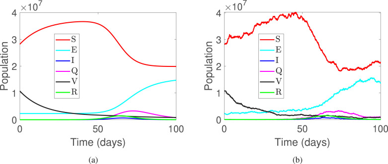
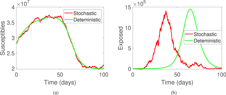
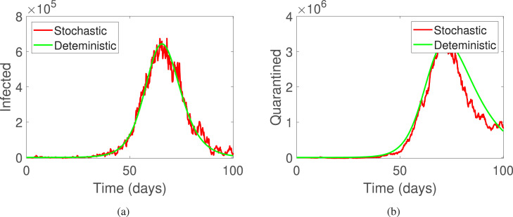
This part of the manuscript presents the numerical simulations along with the discussion on the results obtained. For the simulations, time is considered to be $100$ days and step size as $dt=0.01$. Furthermore, the initial conditions are used to be $\mathrm{S}=28189333,\mathrm{E}=250,\mathrm{I}=110,\mathrm{Q}=2000,\mathrm{V}=10696926,\mathrm{R}=2302039$. The parameters are used as presented in Table 1. In Fig. 1 and Fig. 5, the deterministic and stochastic dynamics of all compartments is presented, where Fig. 1(a) shows deterministic behavior and Fig. 1(b) shows stochastic behavior of the classes of system (2). Further, Fig. 2, Fig. 2 shows the comparison of the stochastic as well as deterministic behavior of susceptible and exposed individuals respectively. Similarly, Fig. 3, Fig. 3 demonstrates the dynamics of infected and quarantined populous. Fig. 4, Fig. 4, are demonstrated to observe the behavior of those individuals who are vaccinated together with the recovered ones.

Table 1.

The parameters and their description of the model (1).

Variables	Description	Value	Source
$\mathcal{A}$	Rate of recruitment	1558	[17]
$\delta$	Coefficient of disease transmission	0.8326	[6]
$k_1$	Rate of vaccination	0.0024	[6]
$\eta$	Immunization by vaccines	0.0643	[6]
${\beta }_1$	Rate of transition from $\mathrm{E}$ to $\mathrm{I}$	0.4127	[6]
${\omega }_1$	Rate of transition from $\mathrm{E}$ to $\mathrm{Q}$	0.1422	[6]
${\omega }_2$	Rate of transition from $\mathrm{I}$ to $\mathrm{Q}$	0.2965	[6]
${\vartheta }_1$	Recovery rate of infected	2864	[6]
${\vartheta }_2$	Recovery rate of quarantined	0.0838	[6]
$\nu$	Mortality rate (natural)	0.0000378	[17]
${\nu }_1$	Mortality rate (COVID related)	0.3394	[6]

Fig. 1.

The population dynamics of all classes of system (1).

Fig. 5.

The population dynamics of all classes of system (1).

Fig. 2.

The deterministic and stochastic population dynamics of susceptible and exposed individuals of system (1).

Fig. 3.

The deterministic and stochastic population dynamics of infected and quarantined individuals of system (1).

Fig. 4.

The deterministic and stochastic population dynamics of vaccinated and recovered individuals of system (1).

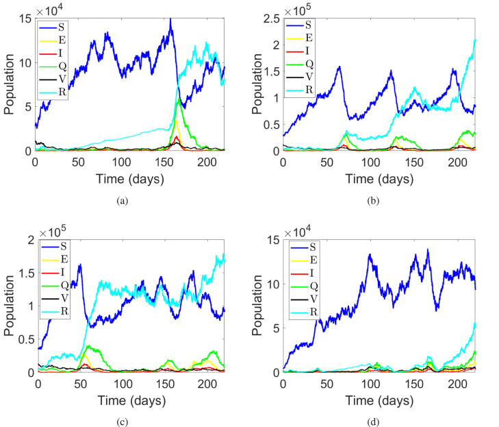
Fig. 6, presents the dynamic of the state variables with a variety of initial conditions to observe the behavior of the system. For this we consider four sets of initial conditions. In the simulation of Fig. 6(a) the initial conditions are considered as $\mathrm{S}=28189,\mathrm{E}=250,\mathrm{I}=110,\mathrm{Q}=2000,\mathrm{V}=10696,\mathrm{R}=2302$, for Fig. 6(b) the initial conditions are used as $\mathrm{S}=30189,\mathrm{E}=1050,\mathrm{I}=2010,\mathrm{Q}=4000,\mathrm{V}=11696,\mathrm{R}=4302$, similarly for Fig. 6(c) the initial conditions are considered as $\mathrm{S}=36189,\mathrm{E}=2050,\mathrm{I}=2510,\mathrm{Q}=6000,\mathrm{V}=12696,\mathrm{R}=5302$ and for the simulation of Fig. 6(d) the initial conditions are supposed as $\mathrm{S}=4189,\mathrm{E}=450,\mathrm{I}=310,\mathrm{Q}=800,\mathrm{V}=1396,\mathrm{R}=1002$. In Fig. 6(a), there is only one wave observed which attains the peak values at $t=160$, while in Fig. 6, Fig. 6 three waves can be seen. Finally in Fig. 6(d), there are several waves with small peaks.

Fig. 6.

The stochastic population dynamics of the different classes individuals in system (1).

The Figs. 7(a), 7(b), and 7(c) depict a comparison of real data from three countries (Iraq, Bangladesh, and Croatia) with simulated results in a stochastic perspective. The data was sourced from [18] and covers the period of 1–30 June 2022 for Iraq and Bangladesh, and 2 September to 1st November 2021 for Croatia, where one unit of time in Fig. 7(c) represents two days. The simulation was carried out over a time span of 30 units with a step size of 0.1, and the parameter $\vartheta$ was set at 0.4864, 6864, and 0.2864 in the simulations of Figs. 7(a), 7(b), and 7(c), respectively. The other parameters used in the simulations are presented in Table 1.

Fig. 7.

The comparison between the real and simulated data of infected individuals from three countries of system (1).

Upon comparing the results, it can be observed that the data is in good agreement with the simulated results, particularly in the case of Iraq and Bangladesh, where almost every data point coincides with the simulated results. This indicates that stochastic behavior plays a crucial role in the analysis of biological models and can provide reliable results.

4.1. Affects of parameters on infections

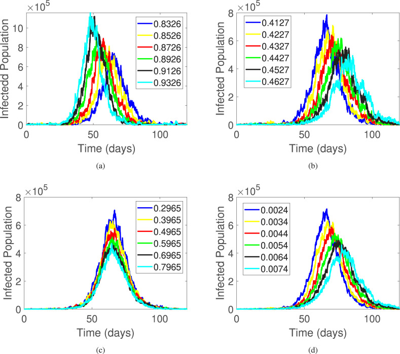
In this section, we examine the dynamics of the infected population in a mathematical model that simulates the spread of COVID-19. We vary four parameters: $\delta$, ${\omega }_2$, ${\vartheta }_1$, and $k_1$, and analyze their effects on number of infections with respect to time. The results are presented in Fig. 8.

Fig. 8.

The dynamics of the infected individuals with varying different parameters in model (1).

First, we examine the impact of a particular parameter, $\delta$, on the spread of the virus, as depicted in Fig. 8(a). The coefficient of disease transmission, represented by $\delta$, has a significant impact on the number of infections within a population. As $\delta$ increases, there is a corresponding increase in the number of infections. For instance, when $\delta$ is equal to 0.8326, the infected population amounts to approximately $7\times 10^5$. However, if we increase $\delta$ to 0.9362, we observe an alarming surge in the number of infections, with the infected population soaring to $11\times 10^5$. This finding highlights the crucial importance of adhering to preventive measures to slow down the transmission of the virus. Measures such as social distancing, mask-wearing, and avoidance of large gatherings are crucial in controlling the spread of the virus. By following these preventive measures, we can minimize the transmission of the disease and consequently reduce the burden on health care systems, which can save countless lives.

Further, we examine the dynamics of the infected population as they recover from the disease and transition from the $\mathrm{I}\left(t\right)$ compartment to the $\mathrm{Q}\left(t\right)$ compartment, with a particular focus on the parameter ${\omega }_2$. The results of this investigation are presented in Fig. 8(b). Specifically, we find that increasing the value of ${\omega }_2$ from 0.4127 to 0.4627 results in a significant reduction in the number of infected individuals, from approximately $8\times 10^5$ to $5\times 10^5$ individuals, respectively. These findings suggest that as more individuals are quarantined, the number of infections decreases, highlighting the effectiveness of quarantine measures in controlling the spread of the virus. These results have important implications for public health policies aimed at managing and mitigating the impact of infectious diseases.

Vaccination has been recognized as one of the most effective tools to control the spread of COVID-19 infections. The COVID-19 vaccines have been shown to reduce the risk of contracting the virus and the severity of symptoms if infected, leading to fewer hospitalizations and deaths. By vaccinating a significant portion of the population, the spread of the virus can be slowed or even halted, as it becomes more difficult for the virus to find new hosts. This not only protects individuals who have been vaccinated but also provides herd immunity to those who cannot receive the vaccine due to medical reasons. Additionally, vaccination can help to reduce the burden on healthcare systems and economies by preventing the overwhelming of hospitals and allowing businesses to operate more normally. Therefore, increasing vaccine coverage remains a critical component of the global efforts to control the COVID-19 pandemic. Now we examine the impact of vaccination and recovery rates on the number of infected individuals. Specifically, we analyzed the influence of the parameters ${\vartheta }_1$ and $k_1$ on the dynamics of the infected population. Our findings, presented in Fig. 8, Fig. 8, demonstrate that increasing the rate of vaccination and recovery can significantly decrease the number of infections. These results emphasize the critical role that vaccination plays in controlling the spread of the virus and reducing the number of cases globally.

Our analysis of the dynamics of COVID-19 transmission underscores the crucial role that transmission reduction and vaccination play in controlling the spread of the virus. By examining the impact of quarantine, vaccination, and recovery rates on the number of infected individuals, we have gained valuable insights into the effectiveness of these measures in mitigating the spread of COVID-19. The implications of our analysis are important for policymakers and healthcare professionals in managing the COVID-19 pandemic and reducing its impact on society. By recognizing the importance of transmission reduction and vaccination, policymakers can develop effective strategies to slow the spread of the virus and mitigate its impact on healthcare systems, economies, and social well-being. Healthcare professionals can also use our findings to inform their decisions regarding the allocation of resources and the implementation of interventions aimed at controlling the spread of the virus.

5. Conclusion

In the this paper, a stochastic model was proposed for COVID-19 that incorporated variables such as incubation times, vaccine effectiveness, and quarantine periods to examine the spread of the virus in symptomatically contagious populations. The conditions needed for a unique global solution of the stochastic model were outlined. Additionally, nonlinear analysis was used to demonstrate some results related to the ergodic aspect of the stochastic model. The model was also simulated and compared to deterministic dynamics. To validate the effectiveness of the proposed system, the paper compared the results of the infected class with actual cases from Iraq, Bangladesh, and Croatia. The data from these countries closely aligned with the dynamics of the infected class, which suggests that the model is valid and applicable to real cases in those countries. Furthermore, the paper visualized the effect of vaccination rates and transition rates on the dynamics of infected people in the infected class. By varying the parameters related to vaccination and transition rates, the evolution of the infected class was altered. This information can aid in predicting the future processes of the COVID-19 epidemic. In conclusion, the proposed stochastic model can provide insight into the dynamics of the COVID-19 epidemic and has the potential to assist in future predictions of the virus.

CRediT authorship contribution statement

Changjin Xu: Formal analysis, Investigation, Writing – original draft, Writing – review & editing. Zixin Liu: Methodology, Funding acquisition. Yicheng Pang: Software, Visualization. Ali Akgül: Data curation, Formal analysis, Software, Writing – original draft.

Declaration of Competing Interest

The authors declare the following financial interests/personal relationships which may be considered as potential competing interests: Changjin Xu reports was provided by Guizhou University of Finance and Economics. Changjin Xu reports financial support was provided by National Natural Science Foundation of China. Changjin Xu reports a relationship with Guizhou University of Finance and Economics - Luchongguan Campus that includes: funding grants. Changjin Xu reports a relationship with Guizhou University of Finance and Economics that includes:. Changjin Xu has patent licensed to Changjin Xu. No

Data availability

No data was used for the research described in the article.

References

- 1.Ghosh J.K., Biswas S.K., Sarkar S., Ghosh U. Mathematical modelling of COVID-19: A case study of Italy. Math Comput Simulation. 2022;194:1–18. doi: 10.1016/j.matcom.2021.11.008. [DOI] [PMC free article] [PubMed] [Google Scholar]
- 2.Vytla V., Ramakuri S.K., Peddi A., Srinivas K., Ragav N.N. Mathematical models for predicting Covid-19 pandemic: A review. J Phys Conf Ser. 2021;1797 [Google Scholar]
- 3.Ahmed I., Modu G.U., Yusuf A., Kumam P., Yusuf I. A mathematical model of coronavirus disease (COVID-19) containing asymptomatic and symptomatic classes. Results Phys. 2021;21 doi: 10.1016/j.rinp.2020.103776. [DOI] [PMC free article] [PubMed] [Google Scholar]
- 4.Kwuimy C.A.K., Nazari F., Jiao X., Rohani P., Nataraj C. Nonlinear dynamic analysis of an epidemiological model for COVID-19 including public behavior and government action. Nonlinear Dynam. 2020;101:1545–1559. doi: 10.1007/s11071-020-05815-z. [DOI] [PMC free article] [PubMed] [Google Scholar]
- 5.Ali Z., Rabiei F., Rashidi M.M., Khodadadi T. A fractional-order mathematical model for COVID-19 outbreak with the effect of symptomatic and asymptomatic transmissions. Eur Phys J Plus. 2022;137:395. doi: 10.1140/epjp/s13360-022-02603-z. [DOI] [PMC free article] [PubMed] [Google Scholar]
- 6.Yavuz Mehmet, Waled Yavız Ahmed Haydar. A new mathematical modelling and parameter estimation of COVID-19: a case study in Iraq. AIMS Bioeng. 2022;9(4):420–446. [Google Scholar]
- 7.Bayat M., Heydari M., Mazdeh M.M. Heuristic for stochastic online flowshop problem with preemption penalties. Discrete Dyn Nat Soc. 2013;2013 [Google Scholar]
- 8.Sohail A., Chighoub F., Li Z. Spectral analysis of the stochastic time-fractional-KdV equation. Alexandria Eng J. 2018;57(4):2509–2514. [Google Scholar]
- 9.Zadorozhniy V.G., Nozhkin V.S., Semenov M.E., Ul’shin I.I. Stochastic model of heat transfer in the atmospheric surface layer. Comput Math Math Phys. 2020;60:459–471. [Google Scholar]
- 10.Sazonov I., Grebennikov D., Meyerhans A., Bocharov G. Markov chain-based stochastic modelling of HIV-1 life cycle in a CD4 T cell. Mathematics. 2021;9(17):2025. [Google Scholar]
- 11.Frei C., Hillen T., Rhodes A. A stochastic model for cancer metastasis: branching stochastic process with settlement. Math Med Biol. 2020;37(2):153–182. doi: 10.1093/imammb/dqz009. [DOI] [PubMed] [Google Scholar]
- 12.Adak D., Majumder A., Bairagi N. Mathematical perspective of Covid-19 pandemic: Disease extinction criteria in deterministic and stochastic models. Chaos Solitions Fractals. 2021;142 doi: 10.1016/j.chaos.2020.110381. [DOI] [PMC free article] [PubMed] [Google Scholar]
- 13.Koufi A., Koufi N. Stochastic differential equation model of Covid-19: Case study of Pakistan. Results Phys. 2022;34 doi: 10.1016/j.rinp.2022.105218. [DOI] [PMC free article] [PubMed] [Google Scholar]
- 14.Din A, Khan A, Baleanu D. Stationary distribution and extinction of stochastic coronavirus (COVID-19) epidemic model, 139, (2020) 110036. [DOI] [PMC free article] [PubMed]
- 15.Faranda D., Alberti T. Modeling the second wave of COVID-19 infections in France and Italy via a stochastic SEIR model. Chaos. 2020;30 doi: 10.1063/5.0015943. [DOI] [PubMed] [Google Scholar]
- 16.Calleri F., Nastasi G., Romano V. Continuous-time stochastic processes for the spread of COVID-19 disease simulated via a Monte Carlo approach and comparison with deterministic models. J Math Biol. 2021;83 doi: 10.1007/s00285-021-01657-4. [DOI] [PMC free article] [PubMed] [Google Scholar]
- 17.Wikipedia. 2022. Available from: https://tr.wikipedia.org/wiki/Koronavir.
- 18.https:www.worldometers.info/coronavirus/countries.
Associated Data
This section collects any data citations, data availability statements, or supplementary materials included in this article.
Data Availability Statement