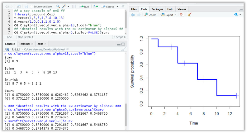
Figure 2.

The R console showing an example of the CG estimator under the Clayton copula. The upper-left panel is the R code. The right panel is the plot of the Clayton CG estimates computed by data $t_i=$ 1, 3, 5, 4, 7, 8, 10, 13; ${\delta }_i=$ 1, 0, 0, 1, 0, 1, 0. The lower-left panel shows the numerical values of the estimates (survival probabilities). The Clayton copula’s parameter is specified as $\alpha =18$ (Kendall’s tau is 0.9). If one specifies the copula parameter as $\alpha =0$, this yields the KM estimator. We see that the numerical results are identical to the results computed by the survfit(.) function (lower-left panel).