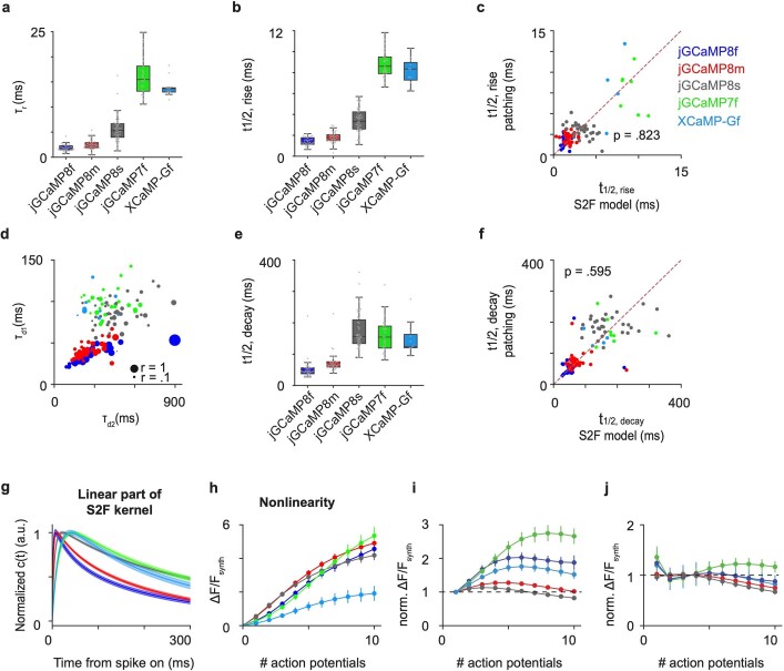
Extended Data Fig. 18. Statistics of S2F fits in the different imaging conditions.

a-f. Statistics of S2F fits in the different imaging conditions (See Extended Data Table 6 for more details). Blue, jGCaMP8f; red, jGCaMP8m; dark gray, jGCaMP8s; green, jGCaMP7f; cyan, XCaMP-Gf. a. Boxplots of rise time constant, τ_r. Minima, 0^th percentile of data (0%); maxima, 100%; center, 50%; bounds of box, from 25% (lower quartile) to 75% (upper quartile); whiskers, 1.5 times the distance between upper and lower quartiles. Number of biologically independent cells collected in each condition is summarized in Extended Data Table 5. b. Boxplots of half-rise time derived from S2F fits. Minima, 0^th percentile of data (0%); maxima, 100%; center, 50%; bounds of box, from 25% (lower quartile) to 75% (upper quartile); whiskers, 1.5 times the distance between upper and lower quartiles. Number of biologically independent cells collected in each condition is summarized in Extended Data Table 5. c. Comparison between half-rise time derived from S2F fits (x-axis) with that measured by super-resolution patch data (y-axis); paired two-sample sign-rank tests; two-sided. Red dashed line is the identity line. d. Scatter plots of decay time constants. X-axis, the slow decay time constant, τ_d2; y-axis, the fast decay time constant, τ_d1; size of dots, the ratio r of the weight for fast decay time to that for the slow one. Number of biologically independent cells collected in each condition is summarized in Extended Data Table 5. e. Box-plots of half-decay time derived from S2F fits. Minima, 0^th percentile of data (0%); maxima, 100%; center, 50%; bounds of box, from 25% (lower quartile) to 75% (upper quartile); whiskers, 1.5 times the distance between upper and lower quartiles. Number of biologically independent cells collected in each condition is summarized in Extended Data Table 5. f. Comparison between half-decay time derived from S2F fits (x-axis) with that measured by super-resolution patch data (y-axis; see Fig. 4e for more details); paired two-sample signed rank tests; two-sided. Red dashed line is the identity line. g, h. ∆F/F_Synth simulated from the S2F models of different sensors. Simulations are based on S2F fits from the biologically independent cells collected in each condition; the number of cells in each condition is summarized in Extended Data Table 5. g. Normalized synthetic calcium latent dynamics, c(t); solid lines, mean; shaded area, s.e.m. h. Simulated peak nonlinearity, i.e., synthetic fluorescence response to different numbers of action potentials. Error bars, s.e.m. across cells. i,j. Measures of linearity of each indicator. Two linear models are shown in i and j. The closer the response curves to 1 (black dashed line, the linear model), the more linear the indicator response is to the number of action potentials. The measure is based on S2F fits from the biologically independent cells collected in each condition; the number of cells in each condition is shown in Extended Data Table 5. i. Normalized peak nonlinearity, where the synthetic fluorescence, $\mathrm{\Delta }F/F\left(nAP\right)$, is normalized as: $\frac{\mathrm{\Delta }F/F\left(\mathit{nAP}\right)}{\mathrm{\Delta }F/F\left(1\mathit{AP}\right)\times n}$, where $\mathrm{\Delta }F/F\left(1\mathit{AP}\right)$ is the peak response to a single action potential, n is the number of action potentials. Error bars, s.e.m. across cells. j. Normalized peak nonlinearity, where the synthetic fluorescence, $\mathrm{\Delta }F/F\left(\mathit{nAP}\right)$, is normalized as: $\frac{\mathrm{\Delta }F/F\left(\mathit{nAP}\right)}{\overline{\mathrm{\Delta }F/F\left(\mathit{nAP}\right)}}$, where $\overline{\mathrm{\Delta }F/F\left(\mathit{nAP}\right)}$ is the linear fit of $\mathrm{\Delta }F/F$ predicted by the number of action potentials n. Error bars, s.e.m. across cells. The linear region (normalized peak nonlinearity is at 1, one-sample Wilcoxon signed rank test, p < .05) for 8s is from 1 to 5 action potentials; that for 8m is from 1 to 6 action potentials; that for 8f is from 3 to 8 action potentials; that for 7f is from 3 to 5 action potentials; that for XCaMP-Gf is from 2 to 8 action potentials.