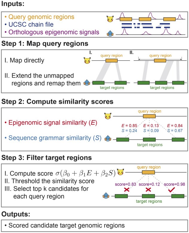
Figure 2.

The AdaLiftOver workflow. The cartoon icons denote any two species with chain files. Top: query regions in the query genome; Bottom: target regions in the target genome. Inputs: genomic coordinates of the query regions, the UCSC chain file from the query genome to the target genome, and the matched epigenome datasets. Step 1: AdaLiftOver defaults to the UCSC liftOver if the query regions map successfully (I). If a query region does not map, AdaLiftOver extends the query region in a local window and applies the UCSC liftOver to this extended query region (II). AdaLiftOver merges small gaps among the resulting orthologous regions and generates candidate target regions based on these merged orthologous regions (indicated by translucent connection bands) with the same width as the query region. Step 2: AdaLiftOver uses local binary epigenomic and sequence grammar feature vectors to compute the similarity scores between the query region and each of the corresponding candidate target regions. Step 3: AdaLiftOver scores the candidate target regions with a logistic model (${\beta }_0=-3,{\beta }_1=4,{\beta }_2=5$) based on their two similarity scores. The users can threshold these scores and rank the candidate target regions based on their probabilities of mapping to the query region. With score threshold of 0.4 or k = 1, AdaLiftOver picks the rightmost candidate target region with estimated probability of mapping as 0.98. Outputs: For each query region, AdaLiftOver outputs a scored and filtered list of candidate target regions that are most similar to the query region in terms of regulatory information