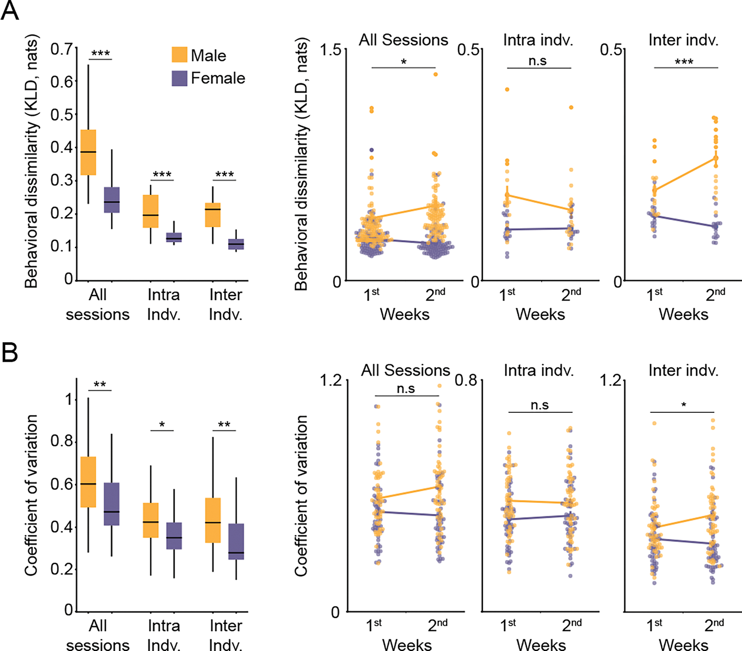
Figure 4: Female behavioral variability is lower than that of males during spontaneous open field behavior.

A) Left: Comparison of male and female behavioral variability, where variability is quantified across all behavioral sessions, across sessions within each individual (intra indv. = intra-individual variability), and across individuals (inter indv. = inter-individual variability) by measuring the KLD of syllable usage distributions. 2-way ANOVA for sex and experimental conditions (exp) as main factors was performed: Fsex(1,438)=55.46, p=5.10*10−13; Fexp(2,438)=16.12, p=1.74*10−7, Fsex*exp(2,438)=1.40, p=0.246. Individual contrasts were performed using student’s t-test with Bonferroni correction: pall sessions=6.42*10−11, nfemale=188 sessions, nmale=192 sessions; pintra-indv=3.3*10−4; pinter-indv=1.28*10−5, n=16 mice for male and females. Right: Variability across the first and second weeks of behavioral assessment (1st: day 1–7, nfemale=93 sessions, nmale=94 sessions; 2nd: day 8–14 nfemale=95 sessions, nmale=98 sessions, excluding the first experimental day in both sexes). Each point represents a single session (for “all sessions” analysis) or a single mouse (for “intra indv.” and “inter indv.” analysis), with mean±sem is presented as lines. 2-way ANOVA for sex and time as main factors was performed for each condition, with individual contrasts using student’s t-test and Bonferroni correction. Significant interaction effects are marked on figure. For all sessions: Fsex(1,376)=46.2613, p=4.08*10−11; Ftime(1,376)=0.90, p=0.34; Fsex*time(1,376)=4.01, p=0.045; For intra-individual: Fsex(1,60)=14.07, p=3.9*10−4; Ftime(1,60)=0.96, p=0.32; Fsex*time(1,60)=1.33, p=0.25; For inter-individual: Fsex(1,60)=73.03, p=5.77*10−12; Ftime(1,60)=3.8, p=0.054; Fsex*time(1,60)=15.23, p=2.4*10−4. Male significantly increased their inter-individual variation between the first and second week of behavioral recordings with p=0.006, all other comparisons were not significant when corrected for multiple comparisons. For visualization purposes (but not analytical purposes) 3 of the 784 data points were excluded because they lie outside the range of the graph. B) Same as in C, but depicted is the coefficient of variation of the usage of each syllable. Each point represents a single syllable, with mean±sem presented as lines. For left panel: 2-way ANOVA: Fsex(1,288)=27.97, p=2.43−7; Fexp(2,288)=42.56, p=6.38*10−17, Fsex*exp(2,288)=0.52, p=0.59. Individual contrasts were performed using student’s t-test with Bonferroni correction: pall sessions=0.0063; pintra-indv=0.015; pinter-indv=0.0051. Right panel: 2-way ANOVA: For all sessions: Fsex(1,192)=17.80, p=3.8*10−−4; Ftime(1,192)=0.7, p=0.39; Fsex*time(1,192)=2.52, p=0.11; For intra-individual: Fsex(1,192)=11.47, p=8.5*10−.4; Ftime(1,192)=0.038, p=0.85; Fsex*time(1, 192)=0.4, p=0.52; For inter-individual: Fsex(1,192)=21.63, p=6*10−6; Ftime(1,192)=0.86, p=0.35; Fsex*time(1,192)=4.04, p=0.045. nmice=16 and nsyllables=49 for both male and females. All individual contrasts were not significant when corrected for multiple comparisons. For all relevant panels, Box plots depict median, interquartile range, and upper/lower adjacent values (black lines). *p<0.05, **p<0.01, ***p<0.001. See also Figure S3, S4 and Table S2.
