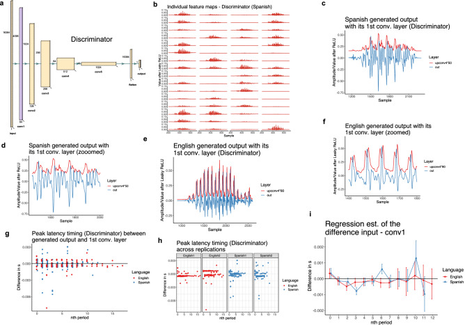
Figure 6.
(a) The structure of the Discriminator network with five convolutional layers66. The first convolutional layer (Conv1) is color-coded with purple. (b) All 64 individual feature maps for a single input (the Generator’s forced output) from the first convolutional layer (Conv1) after Leaky ReLU. (c) One Spanish input (in blue) from the Generator’s forced output with the corresponding values from the first convolutional layer (Conv1) averaged over all feature maps. The plot illustrates peak latency between input and Conv1 for the burst and each vocalic period. (d) A zoomed version of (c) focusing on four vocalic periods. (e) One English input (in blue) from the Generator’s forced output with the corresponding values from the first convolutional layer (Conv1) averaged over all feature maps. The plot illustrates peak latency between input and Conv1 for the burst and each vocalic period. (f) A zoomed version of (e) focusing on five vocalic periods. (g) Raw peak latency timing (input peak time - Conv1 peak time) for burst (=0) and each nth vocalic period across the two conditions (English vs. Spanish). Periods above the 12th period are rare and are discarded from the statistical analysis due to a small number of attestations. The data is pooled across the two replications. (h) Raw peak latency timing across the replications (first and second replication) and two conditions (English and Spanish). (i) Linear regression estimates for the peak latency timing between the two conditions (English vs. Spanish). Periods above the 12th period are discarded from the analysis due to a small number of attestations. The data is pooled across the two replications.

