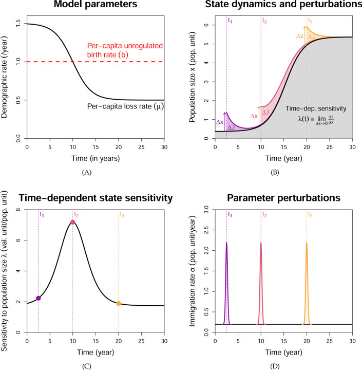
Figure 2: Illustration of time-dependent sensitivity analysis.

(A) We consider an organism in a sink habitat that is being improved through restoration efforts, so the per-capita loss rate µ(t) will eventually fall below the per-capita unregulated birth date b. (B) The population trajectory x(t) is shown in black, and we assume the reward function J is the grey area under the trajectory, plus a terminal payoff (not shown). Now consider a one-off translocation effort to speed up the population recovery at time t. This corresponds to a perturbation x(t) → x(t)+∆x, and leads to a change ∆J in the reward. ∆J can depend on the translocation time t; for example, it is larger at t₂ than at t₁ or t₃. (C) Not surprisingly, the state sensitivity λ(t) is also higher at time t₂. Hence, translocation is most effective right around when µ(t) = b, so the population has just become self-sustaining. (D) Time-dependent parameter sensitivities can be calculated from the state sensitivities. A brief spike in the immigration rate parameter σ at time t produces a state perturbation at time t, and the resulting change in J can be inferred from λ(t). Generalizing this to arbitrary parameter perturbations is straightforward, see Eqn. (A9).