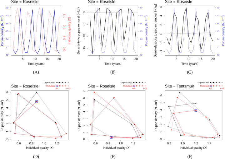
Figure 7: Dynamics and TDSA of the pine looper model.
(A) Oscillatory dynamics in the pine looper, based on parameters estimated for Roseisle forest, Scotland. The blue line indicates pupae density, and the faint red line the average individual quality. (B), (C) The sensitivity and demi-elasticity to culling of pine looper, defined as −λN(t) and −N(t)λN(t) respectively. The reward function here is related to minimizing herbivory damage by the pine looper, see Eqn. (26). The pupae densities are plotted again in faint blue lines to facilitate comparison. (D), (E) Phase plane diagrams when 20% of the moths were culled in Roseisle at t = 4 (a positive demi-elasticity peak) and at t = 6 (a negative demi-elasticity valley). The black and red trajectories indicate the unperturbed and perturbed trajectories. The blue square highlights the start of the perturbed trajectory. (F) Similar to (D), except for the site Tentsmuir at t = 7 (a positive demi-elasticity peak). In (D-F), the differences between the vertical positions of the red and black dots are relevant to the change in reward function.

