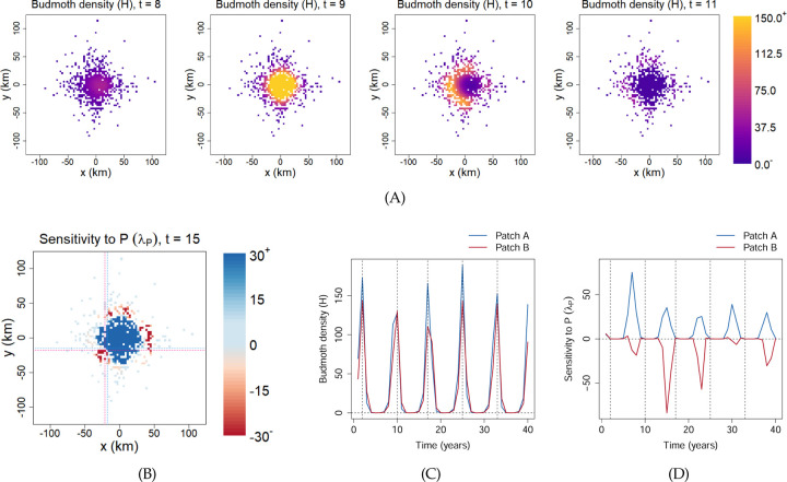
Figure 8: Dynamics and TDSA of the spatially-explicit larch budmoth model.

Each colored pixel corresponds to a suitable habitat patch embedded in a larger landscape. Animated maps of the state variables and sensitivities can be found in the Online Supplement. (A) Snapshots of the budmoth density, showing radial traveling waves. These propagating outbreaks occur every 7–8 years. (B) Snapshot of λ_P, the sensitivity to the addition of parasitoids, at Year 15. We observe a sharp transition from positive to negative values as we move away from the central region. To examine this transition more closely, we selected two adjacent patches, indicated by the intersections of the thin dotted lines (blue–Patch A; red–Patch B). The dynamics of the two patches turn out to be very similar. For example, the budmoth densities peak on the same years as shown in (C). Yet, they show completely different patterns of λ_P in (D): adding parasitoids to Patch A can be beneficial in the right years, but the reverse is true for Patch B. (For reference, the vertical dashed lines indicate the years of peak budmoth densities at the two patches. Also, we have only shown 40 years out of a time horizon of 200 years.) As explained in the main text, this makes it extremely challenging to infer the correct patch-level management actions from the sensitivities alone.