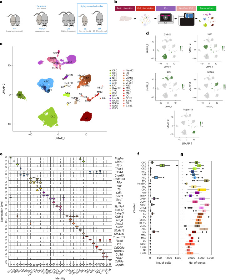
Fig. 1. Overview of the single-cell sequencing analysis.

a, Schematic representation of the animal types used in the present study. Sequencing data from isochronic (YY and OO) and heterochronic (YO and OY) parabiosis pairs were generated and integrated with sequencing data from young (YX) and old (OX) unpaired mice from our previous work³⁷ which were generated simultaneously with those of the parabionts. b, Schematic representation of the experimental workflow (see Methods for details). c, UMAP projection of 105,329 cells across 31 clusters derived from 34 parabionts (7 YY, 9 YO, 7 OO and 11 OY) and 16 unpaired animals (8 YX and 8 OX). For the cell-type abbreviations please see the text and Methods (Supplementary Table 1). d, UMAP projection of five major cell populations showing the expression of representative, well-known, cell-type-specific marker genes (OLGs: Cldn11; ASCs: Gja1; NEUR: Syt1; ECs: Cldn5; MGs: Tmem119). The numbers reflect the number of nCount RNA (UMI) detected for the specified gene for each cell. e, Violin plot showing the distribution of expression levels of well-known, representative, cell-type-enriched, marker genes across all 31 distinct cell types. f,g, Boxplot showing the distribution over n = 50 biologically independent animals of the number of detected cells per cell type (f) or number of detected genes per cell type (g). Boxplot minimum is the smallest value within 1.5× the interquartile range (IQR) below the 25th percentile and maximum is the largest value within 1.5× the IQR above the 75th percentile. Boxplot center is the 50th percentile (median) and box bounds are the 25th and 75th percentiles. Outliers are >1.5× and <3× the IQR. Panel b was created with BioRender.com.