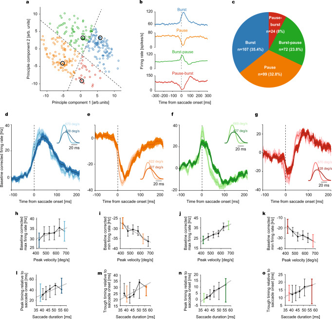
Fig. 3. Classification of simple spike (SS) responses of Purkinje cells (PCs) into different categories and their encoding of saccade kinematics.

a Scatter plot of the first two principal components of SS responses. Classification of PCs into four response categories: burst (blue), pause (orange), burst-pause (green) and pause-burst (red), separated by decision boundaries (dotted black lines). Each data point corresponds to a PC’s SS response in one of the two directions. b Saccade onset-aligned average SS responses of exemplary units taken from each category (large black circles in a). c The proportion of units in each category. d–g SS population response (baseline corrected, mean ± SEM) of all four categories to high and low velocity saccades (see insets for average velocity profiles), represented by lighter and darker shades, respectively. Data are aligned to saccade onset. h–k Baseline corrected, average maximum (h, j) and minimum (i, k) firing rates as a function of saccade peak velocity (bin size = 50 deg/s) for each category. Linear regression parameters: Burst (h): n = 107 units, p = 0.041, R² = 0.69; Pause (i): n = 99 units, p = 0.0068, R² = 0.87; Burst-pause (j): n = 72 units, p = 0.00081 R² = 0.95; Pause-burst (k): n = 24 units, p = 0.0059, R² = 0.88. l–o Average peak (for burst (n = 107) and burst-pause (n = 72) units; l, n) and trough (for pause (n = 99) and pause-burst (n = 24) units; m, o) timing relative to saccade onset as a function of saccade duration (calculated from velocity bins) for each PC category. Linear regression parameters: Burst (l): p = 0.065, R² = 0.61; Pause (m): p = 0.087, R² = 0.56; Burst-pause (n): p = 0.00015, R² = 0.98; Pause-burst (o): p = 0.0059, R² = 0.88. Solid gray lines represent the linear regression fits. Light and dark-colored bins correspond to the high and low peak velocity bins, respectively, for which population responses in d–g are plotted. Data are mean ± SEM.