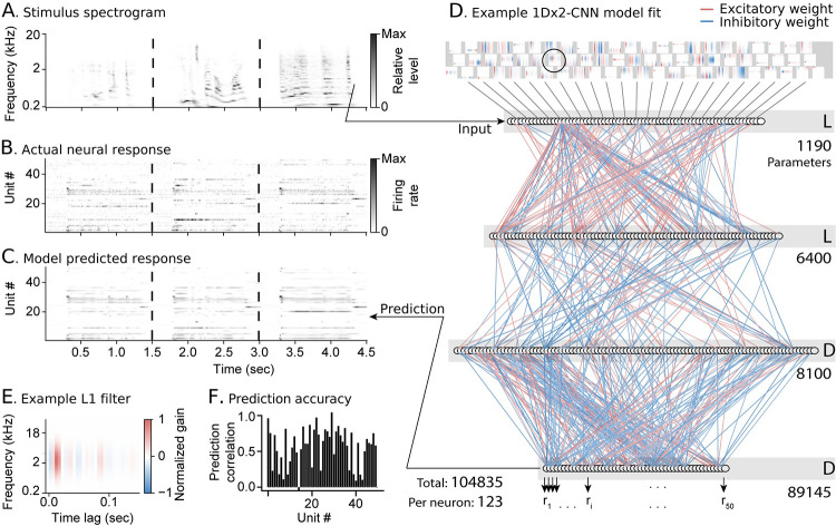
Fig 2. Example population CNN model fit for 849 A1 neurons.
A. Example spectrogram of three natural sounds in the validation set used to measure model performance. B. Heat map shows the actual time-varying spike rate of one neuron per row, for a sample of n = 50 / 849 neurons from the A1 dataset. Spike rate is normalized for each neuron between 0 (white) and maximum (black). C. Heat map of predicted activity for the same units, plotted as in B. D. Schematic of model layers with fitted weights. Convolutional filters in the first layer (top) establish a shared set of spectro-temporal channels. These filters are generated from the outer product of the temporal convolution and spectral summation comprising each 1D convolutional unit. Line color connecting subsequent layers indicates the weight, with positive (excitatory) weights in red and negative (inhibitory) weights in blue. Each unit in the output layer (bottom) predicts the activity of one neuron. The total number of parameters (trainable values) in each layer is listed to the right, with the total number for the model at the bottom left. E. Example filter from the first layer of the population CNN model (circled in D). This filter resembles one typically observed in a standard LN model for a single neuron. F. Prediction correlation for each unit, where unit number corresponds to row in the population raster plots in B-C.

