

Abstract
The aqueous humor actively interacts with the trabecular meshwork (TM), juxtacanalicular tissue (JCT), and Schlemm’s canal (SC) through a dynamic fluid-structure interaction (FSI) coupling. Despite the fact that intraocular pressure (IOP) undergoes significant fluctuations, our understanding of the hyperviscoelastic biomechanical properties of the aqueous outflow tissues is limited. In this study, a quadrant of the anterior segment from a normal human donor eye was dynamically pressurized in the SC lumen, and imaged using a customized optical coherence tomography (OCT). The TM/JCT/SC complex finite element (FE) with embedded collagen fibrils was reconstructed based on the segmented boundary nodes in the OCT images. The hyperviscoelastic mechanical properties of the outflow tissues’ extracellular matrix with embedded viscoelastic collagen fibrils were calculated using an inverse FE-optimization method. Thereafter, the 3D microstructural FE model of the TM, with adjacent JCT and SC inner wall, from the same donor eye was constructed using optical coherence microscopy and subjected to a flow load-boundary from the SC lumen. The resultant deformation/strain in the outflow tissues was calculated using the FSI method, and compared to the digital volume correlation (DVC) data. TM showed larger shear modulus (0.92 MPa) compared to the JCT (0.47 MPa) and SC inner wall (0.85 MPa). Shear modulus (viscoelastic) was larger in the SC inner wall (97.65 MPa) compared to the TM (84.38 MPa) and JCT (56.30 MPa). The conventional aqueous outflow pathway is subjected to a rate-dependent IOP load-boundary with large fluctuations. This necessitates addressing the biomechanics of the outflow tissues using hyperviscoelastic material-model.
Keywords: Trabecular Meshwork, Juxtacanalicular Tissue, Schlemm’s Canal, Hyperviscoelastic, Finite Element Method, Optimization Algorithm
Graphical Abstract

1. Introduction
More than 70% of the aqueous humor exits the eye via the conventional aqueous outflow pathway, comprised of the trabecular meshwork (TM), the juxtacanalicular tissue (JCT), and the inner wall endothelium of Schlemm’s canal (SC) [1–5]. The path of aqueous flow from the anterior chamber to collector channels is shown in Fig. 1. The biomechanical properties of the outflow tissues play a critical role in the regulation of the intraocular pressure (IOP) [6–10]. IOP in the eye is determined through an active outflow resistance in the conventional aqueous outflow pathway that causes a dynamic outflow pressure gradient across the outflow tissues [5, 11–15]. The biomechanical response of the outflow tissues to the dynamic changes in IOP is characterized by morphological changes due to an active, two-way coupling between the outflow tissues and the aqueous humor through a fluid-structure interaction (FSI) mechanism [16, 17]. Hence, the outflow tissues’ motion/displacement and the aqueous outflow resistance [18, 19] partially depend on the biomechanical properties of the outflow tissues [20–25].
Fig. 1.
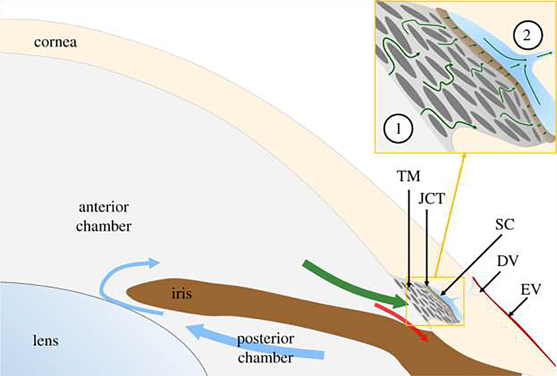
Aqueous humor is secreted into the posterior chamber at a nearly constant rate, enters the anterior chamber through the pupil (blue arrows) and then drains through one of two outflow pathways. The conventional outflow pathway (green arrow) includes the trabecular meshwork (TM), juxtacanalicular tissue (JCT), Schlemm’s canal (SC) and distal vessels (DV), comprising collector channels and intrascleral vessels, leading to episcleral vessels (EV). The unconventional pathway includes flow through the iris root (red arrow) and is believed to be relatively pressure-independent. The circled numbers in the inset refer to the location of the anterior chamber and collector channels. This figure is gotten from Sherwood et al., [110] under CC BY 4.0 license.
In nonhuman primates, rapid fluctuations in intraocular pressure can cause a significant difference of approximately 33 mmHg in less than 0.1 seconds. This rapid change in pressure results in a viscoelastic or rate stiffening effect in the outflow tissues [26, 27]. Previous studies have shown that the outflow tissues [20, 28], which contain collagen fibrils [29, 30], are both anisotropic and viscoelastic, making their mechanical response to dynamic changes in IOP highly dependent on the rate of the applied load. Furthermore, when exposed to large increases in IOP, these tissues exhibit a nonlinear, hyperelastic mechanical response. While linear elastic [22, 31–33] and hyperelastic [34] mechanical properties have been calculated for these tissues in previous studies, the hyperviscoelastic properties of the TM, JCT, and SC inner wall have yet to be determined. We have also calculated the viscoelastic mechanical properties of the TM, JCT, and SC inner wall in the healthy and glaucoma human donor eyes using dynamic SC pressurization in an organ culture prep setup, optical coherence tomography (OCT), and inverse finite element (FE) method coupled with an optimization algorithm [10, 35].
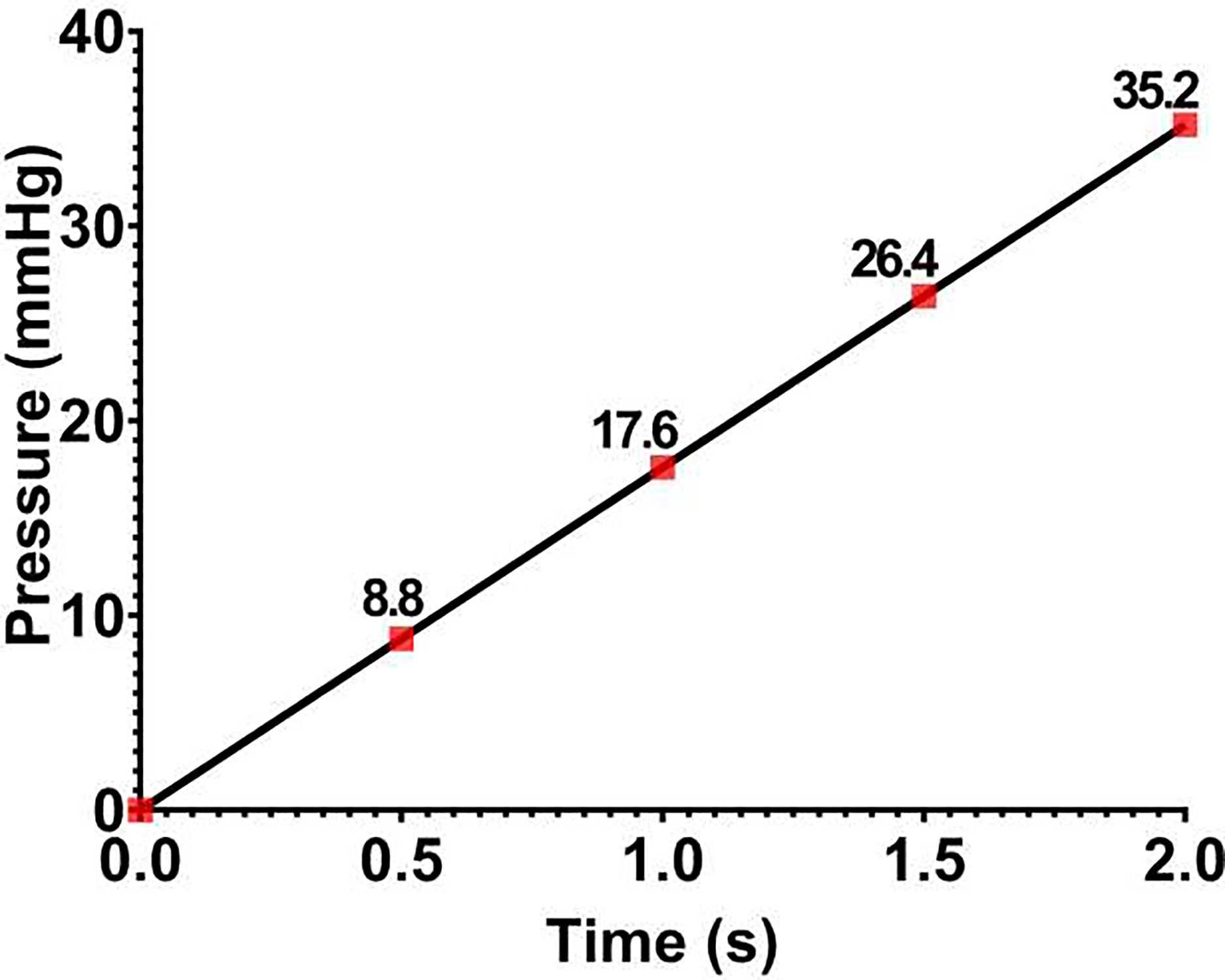
In this study, a quadrant of the anterior segment from a normal human donor eye was pressurized from the SC lumen. Four different pressure boundary conditions were applied on the SC lumen, including 0–8.8, 8.8–17.6, 17.6–25.4, and 25.4–35.2 mmHg, and the dynamic motion of the TM/JCT/SC complex was imaged using a customized OCT setup [36]. The nodal boundaries of the TM, JCT, and SC inner wall in the full stack of OCT images were segmented to reconstruct the 2D geometry and then the 3D extruded FE mesh of the TM/JCT/SC complex [10, 35]. Beam elements that represent the anisotropic distribution of the collagen fibrils in the TM and JCT were distributed in their extracellular matrix (ECM) [35, 37]. The FE method coupled with unconstrained pattern search minimization was then used to adjust the ECM/fiber hyperviscoelastic mechanical properties such that the nodal boundaries in the SC inner wall, SC-JCT junction, JCT-TM junction, and TM edge nodes best matched over pressure steps with the OCT imaging data. The results were represented as the coefficients of the two-parameter Mooney-Rivlin hyperelastic material model (C10 and C01 ) as well as the viscoelastic shear modulus (G) and decay constant (β) for the ECM of the TM, JCT, and SC inner wall. Regarding the viscoelastic material model, the viscoelastic relaxation parameters were the short- (G0), long-time (G∞) shear moduli, and decay constant (β) that were assigned to the collagen fibrils in the TM and JCT. The 3D microstructural FE model of the human outflow pathway in our previous studies was not eye-specific [9, 27], and was reconstructed based on the fixed high-resolution histologic images of the human outflow pathway. However, in this study, the stack of green-light optical coherence microscopy (OCM) images from the same donor eye were used to reconstruct the 3D eye-specific FE model of the outflow tissues. This will significantly help to have more accurate flow analyses using FSI in future studies, so will allow studying the effects of different drugs or treatments on the hydrodynamics of the aqueous humor and biomechanics of the outflow tissues in the conventional aqueous outflow pathway. The FE model, including the TM, with adjacent JCT and SC inner wall, was then subjected to a dynamic SC pressurization load-boundary and the resultant deformation/strain in the outflow tissues were calculated. Finally, a Python/C-based program, TomoWarp2 [38], was used to calculate the resultant deformation/strain in the OCM images of the TM/JCT/SC complex via the digital volume correlation (DVC) method. The resultant deformation/strain from the FSI modeling was validated against the DVC results. The availability of an experimental-computational workflow that facilitates the determination of tissue mechanical properties and subsequent 3D reconstruction of FE models for FSI purposes represents a significant advancement. This approach enables us to investigate the direct impact of drugs on the 3D microstructural geometry and mechanical properties of outflow tissues under dynamic IOP loading conditions. Furthermore, we can employ this approach to compare the 3D microstructural FE models of outflow tissues before and after treatment, thereby providing estimates of changes in trabecular beam morphology induced by a given drug over varying time periods. The determination of tissue mechanical properties before and after treatment using this approach can also lead to a better understanding of the biomechanical changes induced by each drug.
2. Materials and Methods
2.1. Human Donor Eyes, Organ Culture Prep, OCT Imaging, and Green-light OCM Imaging
A healthy human eye (OD) of a 66 year-old (female, Caucasian descent) was obtained within 72 hours postmortem from the Oregon VisionGift eye bank (Portland, Oregon) and the anterior segment was under stationary organ culture conditions [39]. Eye tissue procurement followed the principles of the Declaration of Helsinki.
The anterior segment wedge was dissected, placed interior up, and the SC cannulated as schematically shown in Fig. 2[10, 40]. Briefly, a quadrant of the anterior segment, including the cornea, limbal region with TM, SC, and ~5mm of the sclera, was placed in a petri dish and kept in place with pins. The inner TM surface faced upward, and the entire quadrant was sunken in a saline bath (Fig. 2) [10, 40, 41]. The saline bath also helped to eliminate surface interface motion artifacts because of experimentally induced dynamic TM motion [40]. A cannula was carefully introduced into one end of the SC under the guidance of a dissecting microscope and the other end was sealed with superglue. To ensure a secure seal between the tip of the cannula and the SC lumen, the tip was glued to the inner surface of the canal. This precautionary measure was taken to prevent any potential flow leakage when the pressure inside the SC lumen was raised to 35.2 mmHg. The other end of the cannula was connected to a DMEM (Dulbecco’s Modified Eagle Medium) with HEPES (4-(2-hydroxyethyl)-1-piperazineethanesulfonic acid) buffer reservoir that has relatively the same density as that of the aqueous humor. Pressure in the SC lumen was controlled by altering the height of the reservoirs (Fig. 2).
Fig. 2.
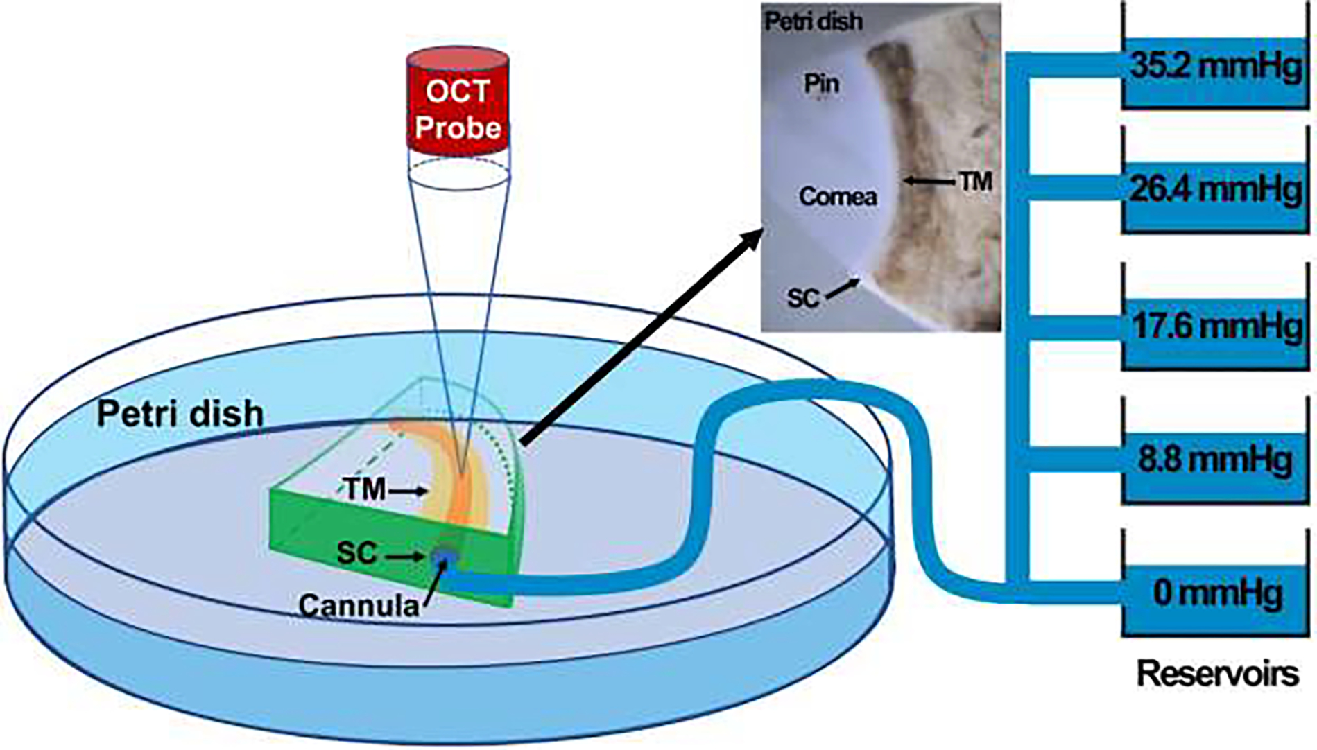
The schematic representation of the experimental setup, including the short-distance OCT and reservoirs to control the pressure in the SC lumen through cannulation from one end of the SC. A quadrant of the donor eye pinned in a petri dish as shown in the inset. This figure is gotten from [10, 35, 111] under CC BY 4.0 license.
To capture a high-resolution dynamic movement of the TM/JCT/SC complex, a customized OCT imaging probe was adjusted to assess enface the TM onto the anterior segment (Fig. 2). While the reservoir heights were increased from 0 to 35.2 mmHg, a series of cross-sectional B-scans through the TM/JCT/SC complex were captured at multiple levels [42]. The spacing between two adjacent B-scans was ~0.75 μm. The OCT images of the TM/JCT/SC complex with the SC pressure of 0 mmHg at four different transversal cross-sectional scans are shown in Fig. 3. The pixel distance through the Z-axis is 4.69 μm, which helps us to cover relatively the entire quadrant, excluding the superglued region [35].
Fig. 3.

(a) The OCT images of the TM/JCT/SC complex at different cross-section. The SC inner wall, SC-JCT, JCT-TM, and TM nodes are shown in this panel. (b) The finite element models of the TM/JCT/SC complex at different cross-section. The SC inner wall, JCT, and TM are shown in this panel. (c) The finite element model of the TM/JCT/SC complex with embedded collagen fibrils. The ECM of the sclera was modeled as hyperelastic neo-Hookean with embedded elastic collagen fibrils. The ECM of the TM and JCT was modeled as hyperviscoelastic with embedded viscoelastic collagen fibrils.
The green-light optical coherence microscopy (OCM) [36] was carried out to image the TM/JCT/SC complex at various pressures and was used for 3D volume reconstruction, FSI modeling, and DVC. The green-light OCM system was based on a spectral domain OCT engine with 510 nm superluminescent diode (~10 nm bandwidth, 9.3-μm axial resolution in tissue). Green-light OCM images were acquired and processed by our custom written graphics processing unit accelerated OCTViewer software package [43, 44]
2.2. Hyperviscoelastic Material Model
In general, in the theory of hyperelasticity, the existence of a Helmholtz free-energy or strain-energy function (per unit reference volume) , with denoting a reference material point (material point in the reference configuration), is postulated in order to characterize the properties of an elastic material. The dependence of on indicates the spatial dependence on the material properties in an inhomogeneous material. For notational brevity, this dependence is omitted henceforth. The strain-energy function may be written as combination of different strain-energy functions which is commonly referred to as additive decomposition. Noting that directional dependent behavior is introduced by a set of collagen fibrils, i.e., with , ubiquitous in different soft tissues, the general form may be written as [45]:
| (1) |
where is the deformation gradient that is given by , where denotes a material point in the current configuration and is the reference gradient operator, , with the indices . The symbol , with , designates the unit mean reference direction of the ith fiber family embedded in the isotopic ground matrix. Local invertibility of the deformation requires that the deformation gradient be non-singular, i.e.,
| (2) |
By virtue of the polar decomposition theorem, the deformation gradient can be written as
| (3) |
where is a proper orthogonal tensor representing a rotation, and and are right and left stretch tensors, both symmetric and positive definite, respectively. The right and left deformation tensors are introduced as:
| (4) |
| (5) |
Furthermore, the following spectral representations are recalled:
| (6) |
| (7) |
| (8) |
| (9) |
| (10) |
| (11) |
where , with , are the principal stretches (will explain in next paragraphs), while and designate the eigenvectors of and and are also known as the reference and current principal axes, respectively. Back to equation (1), the subscripts and distinguish the isotropic and anisotropic parts, respectively. A couple of things are worth highlighting at this point. Firstly, the pure volumetric part of the strain energy function is included in that will be explained more in next paragraphs. Secondly, the term anisotropic is meant in the general sense and also includes transversely isotropic and orthotropic models as special cases. However, herein, the term is not included in our model and instead we have used mesh-free, beam-in-solid material-modeling algorithm (the equations have fully explained previously) to include the directional stiffness due to the collagen fibrils into the TM and JCT’s ECM solid matrix [37].
The hyperviscoelastic material model in our FE code is consisted of a general hyperelastic model that can be combined with a viscoelastic stress contribution. As for the rate independent part, the constitutive law is determined by a strain energy function which can be expressed in terms of the principal stretches, i.e., . To obtain the Cauchy stress, , as well as the constitutive tensor of interest, , they are first calculated in the principal basis after which they are transformed back to the “base frame”, or standard basis. The complete set of formula is given by Crisfield [46, 47] and is for the sake of completeness recapitulated here.
The principal Kirchoff stress components are given by:
| (12) |
that are transformed to the standard basis using the standard formula:
| (13) |
The are the components of the orthogonal tensor containing the eigenvectors of the principal basis. The Cauchy stress is then given by:
| (14) |
where is the relative volume change as also previously described.
The constitutive tensor that relates the rate of deformation to the Truesdell (convected) rate of Kirchoff stress can in the principal basis be expressed as in:
| (15) |
These components are transformed to the standard basis according to:
| (16) |
and finally the constitutive tensor relating the rate of deformation to the Truesdell rate of Cauchy stress is obtained through:
| (17) |
The strain energy function for the general hyperelastic model is given by:
| (18) |
where is the bulk modulus,
| (19) |
and
| (20) |
are the first, second, and third invariants of the unimodular components of the Cauchy-Green tensor in terms of the principal stretches. To apply the formulas in the previous equations, we require:
| (21) |
where
| (22) |
if is nonzero only for , equation (21) can be written as:
| (23) |
Proceeding with the constitutive tensor, we have:
| (24) |
where
| (25) |
Again, using only the nonzero coefficients mentioned above, equation (24) is reduced to:
| (26) |
which is the general or polynomial form of the hyperelastic strain energy function. In this study, the Mooney-Rivlin or 2nd order form of the above equation was used that includes only the and , so the , , , and were set to zero. Thus, the equation (26) can be written as:
| (27) |
considering equation (25), the equation (27) can be written as:
| (28) |
and this was used to address the general hyperelastic mechanical properties of the tissues. As mentioned above, the material model is also accompanied with a viscoelastic stress contribution. The rate form of this constitutive law can in co-rotational coordinates be written as:
| (29) |
Here is a number less than or equal to 6 (based on the series order, here we chose 1), is the co-rotated viscoelastic stress, is the deviatoric co-rotated rate-of-deformation and and are material parameters. The parameters can be thought of as shear moduli and as decay coefficients determining the relaxation properties of the material. The rate form can be integrated in time to form the co-rotated viscoelastic stress [47]:
| (30) |
For the constitutive matrix, we refer to
| (31) |
It should be noted that the hyperviscoelastic material model herein allows us to address the rate dependency and the large-deformation biomechanical responses of the outflow tissues simultaneously.
The viscoelastic material model was used to address the mechanical properties of the collagen fibrils in the TM and JCT. In this model, linear viscoelasticity is assumed for the deviatoric stress tensor as follows [48]:
| (32) |
where
| (33) |
is the shear relaxation modulus. and are the short- and long-time shear moduli, respectively. The is the decay constant [49].
The , , , and are the input parameters for the tissues’ ECM and the , and are the input parameters for the collagen fibrils that are determined using finite element method coupled with an unconstrained pattern search minimization algorithm as will be explained in the next section. The shear modulus in the two-parameter Mooney-Rivlin hyperelastic material model is defined as . The ECM/fibrils were treated as nearly incompressible with the Poisson’s ratio of 0.495 [9, 10, 27]. The collagen fibrils in the sclera was modeled as a simple elastic material model. It should be noted that the shear modulus with the term “” is used to define the hyperelastic material model while “” is used for the same purpose in the viscoelastic material model.
2.3. TM Specimen and Inverse Finite Element Method
The hyperviscoelastic parameters that we calculate in this section for a TM specimen FE model will be used as the initial guess for the inverse FE-optimization algorithm in section 2.4
We pre-estimated the hyperviscoelastic properties of the FE model using a TM specimen from a normal human TM tested in tension [50]. The FE model of the TM specimen of 10 mm length × 0.24 mm width × 0.136 mm thickness equals the specimen dimensions in the experimental study [50] as shown in Fig. 4a. Anisotropic and viscoelastic collagen fibrils were incorporated in the TM FE model and coupled with the hyperviscoelastic ECM using a mesh-free, beam-in-solid material modeling algorithm [37]. The TM FE model was subjected to a uniaxial tensile strain, where the displacement boundary condition (2% strain) was applied to the FE model to mimic the uniaxial mechanical testing protocol [50]. The unconstrained pattern search minimization was coupled with the LS-DYNA (Ansys/LS-DYNA, Pennsylvania, US) solver to calculate the hyperviscoelastic parameters for the ECM with embedded viscoelastic collagen fibrils [10, 51, 52]. This algorithm minimizes an unconstrained problem using the pattern search solver. The hyperelastic two-parameter Mooney-Rivlin coefficients ( and ) for the TM were calculated based on the healthy human TM nominal/engineering stress-strain data [50]. These parameters were then used as initial estimations for the optimization algorithm. The optimization algorithm started with initial estimations of (average of the shear modulus based on our prior publication [35]), and the constant (decay constant) =109 1/s [35] for the hyperviscoelastic ECM of a healthy human eye. The optimization algorithm also started with initial estimations of (short-time shear modulus) =36.19MPa, (long-time shear modulus) =19.58 MPa, and the constant (decay constant) =4501/s for the viscoelastic collagen fibril of a healthy human eye [35]. The upper and lower parameter boundaries for both the ECM/fibrils were chosen as , , , , , and always to have a positive shear modulus for the tissues [10, 35]. The model was run in Matlab (Mathworks, Natick, Massachusetts, US) with the cost function of mean squared error [53] that is the sum of the squared differences between the experimental data [50] and optimized value. The resultant stress-strain in the gauge at the center of the TM specimen FE model (Fig. 4a) was calculated and plotted versus the experimental data [50, 54] as presented in Fig. 4b. The optimized material properties for the ECM/fibrils FE model are summarized in Table 1.
Fig. 4.
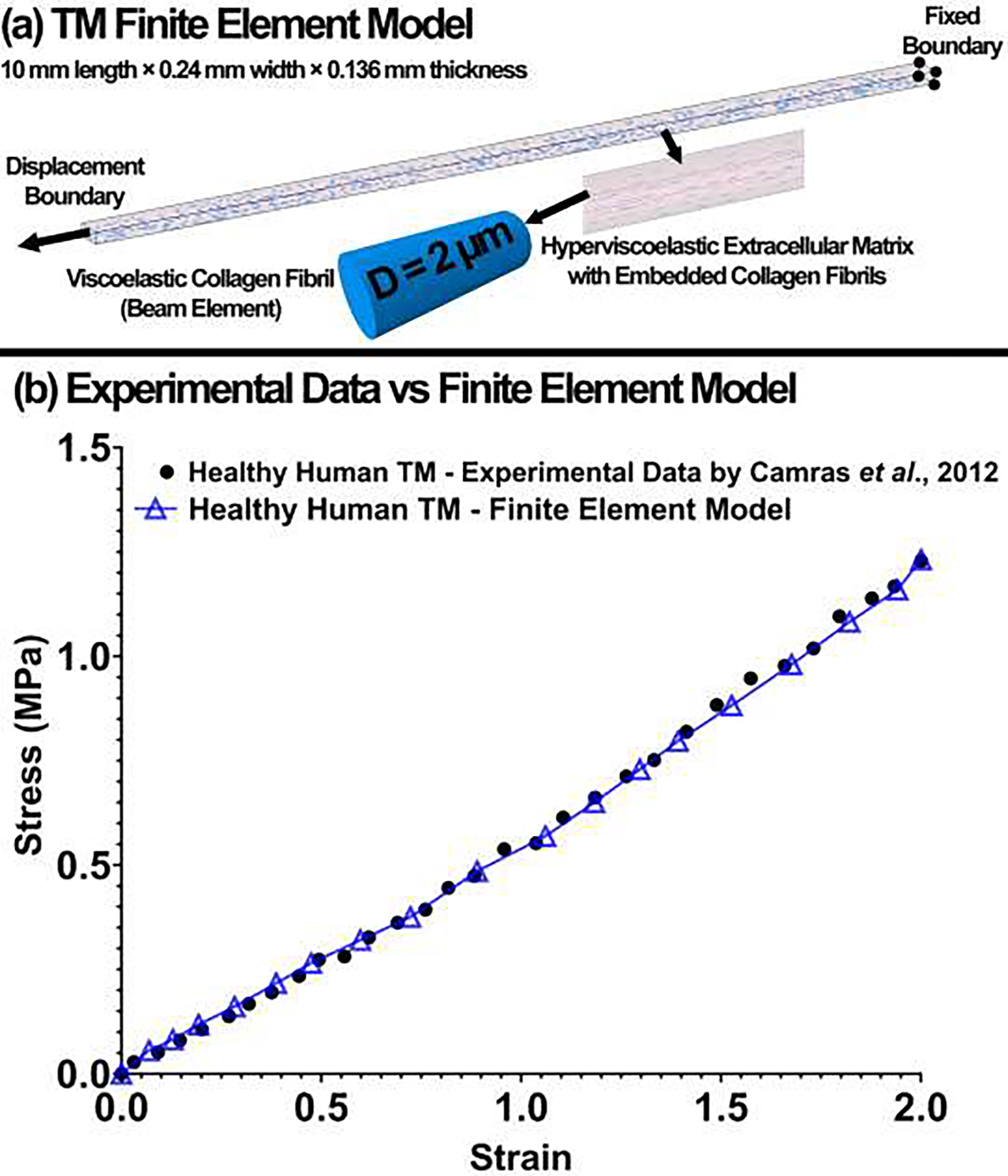
(a) The TM finite element model. The ECM of the TM was modeled as hyperviscoelastic with embedded viscoelastic collagen fibrils. The displacement boundary condition was applied on one end of the TM FE model and the other end was fixed. (b) The experimental stress-strain data versus finite element model for the healthy human TM.
Table 1.
Hyperviscoelastic parameters for the TM FE model with embedded viscoelastic collagen fibrils.
| Hyperviscoelastic Parameters | C10 (MPa) | C01 (MPa) | G (MPa) | β (1/s) |
| Extracellular Matrix | 3.65 | −3.60 | 56.29 | 109 |
| Viscoelastic Parameters | G0 (MPa) | G∞ (MPa) | β (1/s) | |
| Beam Element | 66.2 | 52 | 450 |
2.4. TM, JCT, SC Inner Wall Segmentation, Volume Meshing, and Inverse Finite Element Method
The flow-chart of the OCT imaging, the TM, JCT, and SC inner wall boundary segmentation, nodal coordinates extraction, and optimization process to calculate the hyperviscoelastic mechanical properties of the ECM and viscoelastic properties of the collagen fibrils are shown in Fig. 5. The OCT with 80 B-scans/second at an appropriate distance from the cannula provided a set of dynamic images of the TM/JCT/SC complex as the pressure in the SC elevates from 0 to 8.8, 8.8 to 17.6, 17.6 to 26.4 , and 26.4 to 35.2 mmHg. The TM/JCT/SC complex segmentation and volume meshing are fully explained in our prior publications [10, 35]. The TM, JCT, and SC inner wall were segmented in the OCT images [52] under the supervision of an expert glaucoma specialist as shown in Fig. 3a. The nodal boundaries in the TM/JCT/SC complex were used to define the cost function for the material properties calculation using inverse FE method.
Fig. 5.
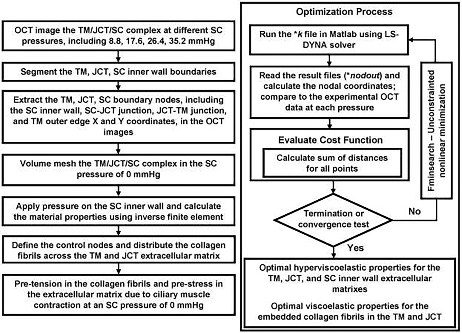
Flow-chart of the imaging, segmentation, finite element model reconstruction, and inverse finite element coupled with an optimization algorithm.
The nodal coordinates in the SC inner wall, JCT, and TM boundaries were imported into a custom Matlab code to reconstruct the geometry of the TM/JCT/SC complex. To reduce the sharp vertices in the final FE mesh, the boundaries of the TM/JCT/SC complex were smoothed [10] using a smoothing spline algorithm [55]. The output file as *igs (initial graphics exchange specification) was imported to LS-DYNA, extruded to 10-μm thickness, and volume meshed [56] using an 8-noded hexahedral element type with fully integrated element formulation as shown in Fig. 3b. The control points were distributed into the TM and JCT’s solid matrix (surface mesh *STL stereolithography) using a custom Matlab program for further collagen fibrils’ distribution [37]. The distance between the control points was set to 2.5 μm (planar) and 2.5 μm (through the thickness) that is limited by the 10-μm thickness of the model. The collagen fibrils were distributed in an asymmetric fan-shaped configuration parallel to the external and internal edges of the TM [5, 41, 57–63] using a custom Matlab program as shown in Fig. 3c. The motion/rotation of the collagen fibrils in the space is controlled by the ECM as they are fully coupled through a mesh-free, beam-in-solid material modeling algorithm [37]. The collagen fibrils or beam elements can only understand the tension when the applied load-boundary in the TM or JCT’s ECM aligns in the direction of the collagen fibrils. The sclera with the same thickness of 10-μm and the length of half of the length of the TM/JCT/SC complex in the X direction was added to the model. The elastic collagen fibrils were incorporated into the ECM of the sclera as indicated in Figs. 3c. The neo-Hookean hyperelastic and elastic material models were assigned to the scleral’s ECM and collagen fibrils, respectively [37, 56]. The pressure boundary was applied on the SC inner wall based on the organ culture prep experiment explained in section 2–1. The solid TM, JCT, and SC inner wall extracellular matrixes were modeled as a hyperviscoelastic material using 8-noded hexahedral elements with mesh-free Galerkin formulation [64, 65]. The mesh-free Galerkin formulation allows us to distribute the collagen fibrils in the ECM independent of the TM and JCT’s element shape, so it presents a more realistic and physiological distribution for the collagen fibrils.
The unconstrained pattern search minimization algorithm was coupled with the LS-DYNA finite element solver to calculate the hyperviscoelastic parameters for the ECM of the TM, JCT, and SC inner wall as well as the viscoelastic parameters for the embedded collagen fibrils in the ECM of the TM and JCT. The initial estimations for the ECM of the TM, JCT, and SC inner wall were , , MPa, and constant 1/s (Table 1). For the viscoelastic collagen fibrils in the ECM of the TM and JCT, the initial estimations were , with a constant (Table 1). The upper and lower parameter boundaries for the ECM/collagen fibrils were , , , , and MPa considering always to ensure a positive shear modulus for the ECM of the outflow tissues. The models were run with the cost function of mean squared error between the SC inner wall, SC-JCT, JCT-TM, and TM edge nodal coordinates of the OCT experimental data and optimization data. The optimized hyperviscoelastic properties for the TM, JCT, and SC inner wall as well as the viscoelastic properties for the collagen fibrils are summarized in Table 2.
Table 2.
Hyperviscoelastic parameters for the TM, JCT, and SC inner wall. Viscoelastic parameters for the collagen fibrils embedded in the extracellular matrix of the TM and JCT.
| Cross-section #1 | ||||
|
| ||||
| Hyperviscoelastic Parameters | C10 (MPa) | C01 (MPa) | G (MPa) | β (1/s) |
|
| ||||
| TM | 7.87 | −6.92 | 51.97 | 109 |
| JCT | 6.58 | −6.13 | 35.95 | 109 |
| SC inner wall | 1.20 | −0.47 | 99.89 | 109 |
|
| ||||
| Viscoelastic Parameters | G0 (MPa) | G∞ (MPa) | β (1/s) | |
|
| ||||
| Collagen fibrils (TM) | 122 | 27.07 | 450 | |
| Collagen fibrils (JCT) | 118 | 21.67 | 450 | |
|
| ||||
| Cross-section #2 | ||||
|
| ||||
| Hyperviscoelastic Parameters | C10 (MPa) | C01 (MPa) | G (MPa) | β (1/s) |
|
| ||||
| TM | 7.93 | −6.98 | 99.97 | 109 |
| JCT | 6.75 | −6.26 | 67.88 | 109 |
| SC inner wall | 1.20 | − 0.47 | 99.95 | 109 |
|
| ||||
| Viscoelastic Parameters | G0 (MPa) | G∞ (MPa) | β (1/s) | |
|
| ||||
| Collagen fibrils (TM) | 121.07 | 31.07 | 450 | |
| Collagen fibrils (JCT) | 100.55 | 11.45 | 450 | |
|
| ||||
| Cross-section #3 | ||||
|
| ||||
| Hyperviscoelastic Parameters | C10 (MPa) | C01 (MPa) | G (MPa) | β (1/s) |
|
| ||||
| TM | 7.87 | −7.05 | 87.29 | 109 |
| JCT | 6.81 | −6.36 | 86.70 | 109 |
| SC inner wall | 1.75 | −1.05 | 92.39 | 109 |
|
| ||||
| Viscoelastic Parameters | G0 (MPa) | G∞ (MPa) | β (1/s) | |
|
| ||||
| Collagen fibrils (TM) | 138.2 | 36.20 | 450 | |
| Collagen fibrils (JCT) | 130.8 | 18.20 | 450 | |
|
| ||||
| Cross-section #4 | ||||
|
| ||||
| Hyperviscoelastic Parameters | C10 (MPa) | C01 (MPa) | G (MPa) | β (1/s) |
|
| ||||
| TM | 7.87 | −6.92 | 98.29 | 109 |
| JCT | 6.25 | −5.76 | 34.70 | 109 |
| SC inner wall | 1.00 | 0.27 | 98.39 | 109 |
|
| ||||
| Viscoelastic Parameters | G0 (MPa) | G∞ (MPa) | β (1/s) | |
|
| ||||
| Collagen fibrils (TM) | 130.20 | 24.80 | 450 | |
| Collagen fibrils (JCT) | 123.20 | 21.20 | 450 | |
|
| ||||
| Average of 4 cross-section | ||||
|
| ||||
| Hyperviscoelastic Parameters | C10 (MPa) | C01 (MPa) | G (MPa) | β (1/s) |
|
| ||||
| TM | 7.88 | −6.96 | 84.38 | 109 |
| JCT | 6.59 | −6.12 | 56.30 | 109 |
| SC inner wall | 1.28 | −0.43 | 97.65 | 109 |
|
| ||||
| Viscoelastic Parameters | G0 (MPa) | G∞ (MPa) | β (1/s) | |
|
| ||||
| Collagen fibrils (TM) | 127.86 | 29.78 | 450 | |
| Collagen fibrils (JCT) | 118.13 | 18.13 | 450 | |
It should be noted that the unconstrained pattern search minimization algorithm finds the minimum of an unconstrained multivariable function through the derivative-free method [66]. In such optimization/minimization algorithm, uncertainty is an inevitable part of the solution [67]. Thus, the optimized material properties that we have reported in Tables 1 & 2 may not be an absolute minimum but we can say they are the best possible minimum solution that were achieved after more than ~300 iterations (300-run in Matlab workspace using LS-DYNA FE solver). To avoid or eliminate the non-unique solutions from the optimization problem, wise selection of the initial estimations along with the reasonable limitations may significantly help [68, 69]. In this study, we limited the parameters with suitable physiologically possible upper and lower bounds [10]. We also perturbed the system by selecting different initial estimations [66, 69], with 10%, 20%, 30%, and 40% larger and smaller values compared to the optimized material parameters. The converged properties were then compared to those of the optimized set of parameters (Tables 1 & 2). In all simulations, optimization resulted in similar parameters (less than ~7% difference), so we can say that the solution is robust.
2.5. TM/JCTISC Compiex FE Mesh, Hydraulic Conductivity, Fluid-Structure Interaction, and Boundary Condition
An original grayscale cross-section of the TM/JCT/SC complex in a typical OCT image is shown in Fig. 6a. The grayscale image was converted to a binary image as shown in Fig. 6b. The bright-line saturated artifact in the original grayscale images was manually eliminated throughout the entire stack of OCT images. An image-to-mesh algorithm was employed to volume-mesh the OCT images [56] as shown in Fig. 6c–d. The binary images of the TM/JCT/SC complex (Fig. 6b) were stacked in a volume representing the entire TM/JCT/SC complex microstructure. The images were stacked to construct a triangular isosurface image volume using a constrained Delaunay approach as shown in Fig. 6c–d. Since the isosurface was not closed, the surface edges located on the bounding box of the volume were calculated and a piecewise linear complex was added to form a closed surface using a free Iso2Mesh library [70, 71]. The triangular surface meshes were directly generated from the input isosurface volume using a modified surface extraction program built on a free library, CGAL [72]. A mesh repairing process based on a surface simplification approach was applied to the resulting surface to remove topological complications, such as isolated vertices, duplicated triangles, and nonmanifold vertices [73]. Since these shortcomings may lead to a cascade of difficulties with final mesh generation, a customized Matlab script based on the free JMeshLib library [73], was used to find the non-manifold vertices and repair them by replication. The input volume may contain multiple sub-regions of the TM/JCT/SC complex, so correctly tagging the resulting 3D finite elements with the associated region is critical for the FE analyses. The determination of an interior point for each sub-region in a volumetric image could be a solution; however, it is not a trivial task because the extracted isosurfaces are not necessarily convex. A distance-field method was used to robustly determine an internal point for each sub-domain. First, all the edge voxels of each sub-domain were identified then set to 1 inside the boundary and 0 elsewhere. Thereafter, a Gaussian smoothing kernel (smoothing factor ) was applied for 10 iterations to the resulting array using a custom Matlab script [56]. This produced a 3D field where the values are inversely related to the distances from the domain boundaries. The application of this method assures that the resulting points are located strictly inside the specified sub-regions and are roughly (depending on the geometry of the model) voxels away from the boundaries. Here, an or 4 was found to work robustly for outflow tissues with only minimal additional computation. Since our model contained pore regions, these regions were simply tagged with a label and the same algorithm was applied to determine the interior points. These regions were eventually removed from the final mesh using their regional labels. It was important to ensure that the surfaces constructed from the binary images did not have openings or holes, especially at their peripheral boundaries. Here, we developed an approach that assumed that the edges of the open surfaces are all located inside the volume-bounding box, and thus piecewise linear complexes on the bounding box are needed to enclose the surfaces. All open edges of the surfaces were computed and then organized into a list of disjointed loops to generate water-tight surfaces. If a loop crossed the intersections of two or three bounding box faces, it was further decomposed into sub-loops that conform to a single face. A regional exclusion algorithm was then applied to flatten the bounding faces by the polygons enclosed by the edge loops. The final meshed TM/JCT/SC complex microstructure is shown in Fig. 6c–d. Thereafter, parent volume-mesh with 8-noded hexahedral elements (fully integrated) having the element edge length of ~0.5 μm, and the same dimensions as that of the TM/JCT/SC complex volume-mesh was reconstructed and translated to the same coordinate system as that of the microstructural FE mesh of the TM/JCT/SC complex (Fig. 6c–d). Because the element edge length of the reconstructed FE mesh is ~0.5 μm that is smaller than the pixel size (voxel resolution) of the OCT images (0.75 μm), the mesh density analyses were performed. This helped us to ensure the resultant strains in the outflow tissues are independent of the number of the elements [9, 27]. A meshing algorithm was then used to separate the parent volume mesh to the TM, JCT, SC inner wall with interspersed aqueous humor [9, 27, 56, 74]. The boundary overlay comparison between the 3D reconstructed microstructure of the TM/JCT/SC complex and the OCT images at several (~10) cross-section was done to ensure the accuracy of the FE models [9, 56]. The TM/JCT/SC complex FE mesh includes the TM, with adjacent JCT (~5-μm) [75] and SC inner wall (~2-μm) [12] regions. Micrometer-sized pores were distributed in the SC inner wall [76], with a pore density and diameter of 835 pores/mm2 [12] and 1.3-μm [77], respectively. The final model is shown in Fig. 7a. The mesh-free, beam-in-solid material modeling algorithm [35] was used to distribute the viscoelastic beam elements into the ECM of the TM and JCT to model the directional stiffness imparted by the anisotropic collagen fibril orientation in those tissues [78–80] as indicated in Fig. 7b. The elastic collagen fibrils were also distributed in the ECM of the sclera [37, 56]. The 3D microstructural FE model was subjected to the same loading condition (Fig. 7) from the SC inner wall as that of the SC pressurization experiment.
Fig. 6.
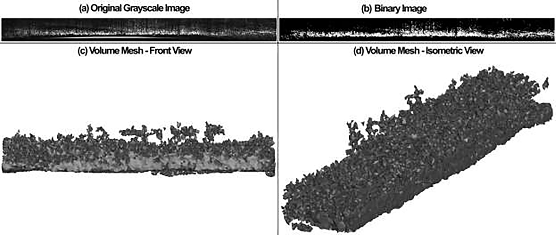
(a) The original grayscale and (b) binary OCT image of the TM/JCT/SC complex. The volume mesh of the TM/JCT/SC complex from the (c) front and (d) isometric views. Element edge length of ~1μm.
Fig. 7.
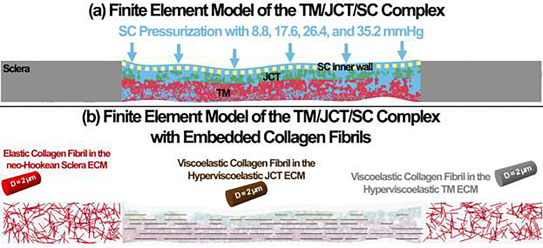
(a) The finite element model of the TM/JCT/SC complex (b) with embedded collagen fibrils. The ECM of the sclera was modeled as hyperelastic neo-Hookean with embedded elastic collagen fibrils. The ECM of the TM and JCT was modeled as hyperviscoelastic with embedded viscoelastic collagen fibrils.
The hydraulic conductivity, which is defined as how easily pore fluid escapes from the compacted pore space, is responsible for ~10% of total outflow resistance [81, 82]. The hydraulic conductivity of 2.0 μl/min/mmHg/cm2 [83], 2.5 mmHg/μl/min/cm2 [84], and 9000×10−11 cm2 sec/g [85] were programmed for the TM, JCT, and SC inner wall ECM, respectively, through a custom subroutine in LS-DYNA [9, 27].
Regarding the FSI, the solid and fluid domains that are representing the TM/JCT/SC complex (Lagrangian) and aqueous humor (Eulerian) [9, 27, 35], respectively, were defined using an arbitrary Lagrangian-Eulerian (ALE) method [86, 87]. The multi-material ALE (Ansys/LS-DYNA, Pennsylvania, US) automatic mesh refinement algorithm was used to enhance the modeling accuracy through the Lagrangian and Eulerian mesh motions within the same framework [88, 89]. The flow in the organ culture prep perfusion system that has similar properties to that of the aqueous humor was simulated as homogeneous, Newtonian, and viscous [90], with the density and dynamic viscosity of 1000 kg/m3 and 0.7185×10⁻³ Pa·s [91], respectively.
Deformable fluid and solid domains can be explained through the ALE approach wherein the fluid mesh is updated to follow the structure’s motion [86, 87]. The “ALE incompressible” material was used with the element formulation of “one-point ALE multi-material group” to address the fluid properties [92]. Briefly, three domains were defined as spatial, material, and reference. The Eulerian reference was achieved through the coincidence of the spatial domain and the reference domain. The Lagrangian reference was obtained through the coincidence of the material domain and the reference domain. Since both the material and spatial domains with respect to the reference domain are in motion, the material time derivative of a physical property in the reference configuration can be defined as [93]:
| (35) |
where is the material time derivative, and is the time derivative when the coordinates in the reference domain are fixed. The convective velocity, , is defined as:
| (36) |
where is the fluid velocity and is the mesh velocity. In the Eulerian reference, the mesh velocity is zero , while in the Lagrangian reference and .
The Lagrangian formulations were used to solve the solid TM, JCT, and SC inner wall problems that displacement of the nodes and the elements on a Lagrangian mesh correspond to the movements of aqueous humor (fluid). The edges of the ALE fluid mesh always coincide (node-to-node) with the edges of the solid elements. In the Cartesian coordinate system, the displacement of the solid in a domain is governed by:
| (37) |
with the initial and boundary conditions of:
| (38) |
Where T is the end-time for the incremental solution. The movement of the fluid was addressed through the Eulerian approach where the movement of the fluid was solved in fixed positions so that the domain of study was fixed and the fluid was updated constantly in each load increment. This method introduces a convection term into the equations and avoids large distortions of the mesh. Thus, an ALE method that combines the Eulerian and Lagrangian descriptions at the same time was used to address the movement of the fluid. The mass and momentum conservation laws can be defined as:
| (39) |
| (40) |
where and are the flow velocity and density, respectively. The term indicates the velocity of the mesh. If , the Eulerian formulation will be achieved as the convective velocity of the mesh is null. If , the Lagrangian formulation will be achieved as the convective velocity is equivalent to the fluid velocity. The quantity is the relative velocity and the stress tensor , commonly defined by:
| (41) |
where is the fluid dynamic viscosity.
The momentum equations is solved with the initial and boundary conditions as follows:
| (42) |
| (43) |
where are the imposed velocity components on .
The boundary conditions on the FSI surface are defined as:
| (44) |
And , on the outflow boundary [94]
Penalty coupling was also defined between the fluid and solid elements as normal direction to account for both the compression and tension at the interaction site. The penalty factor that scales the calculated stiffness of the interacting (coupling) system was set to 0.1[90, 95–98].
A 20-core Intel ® Xeon® CPU W-2155@3.30 GHz computer with 256GB RAM was used to run the FSI simulation in dynamic-explicit LS-DYNA. The loading was applied in 2 sec with the time-step of 0.1 (20 time-step). The same time-step was used for both the FE-optimization algorithm and FSI simulations to make sure the effect of pressure-rate is similar in both simulations. The FSI simulation on average took ~382 hours to run on our workstation.
2.6. Digital Volume Correlation
A Python/C-based code, namely TomoWarp2 [38], was used to calculate the resultant displacement across the TM/JCT/SC complex in the volumetric OCT images at different SC pressures, including 0–8.8, 0–17.6, 0–26. 4,0–35.2mmHg. The program allows the measurement of 3D vector displacement fields between two volume images over a 3D grid of points. The input file to the code was a stack of OCT images in the reference (un-deformed) and deformed configurations. The images were treated with a median filter of size 2 pixels before the analysis. Cubic subsets of 5 pixels per side and a node spacing of 15 pixels were used for displacement calculation. The complete 3D tensor strain field was then calculated from the gradients of the DVC displacements. The original OCT image was median filtered and the outlier was removed [38] as shown in Fig. 9. The region of interest in the OCT images, including the TM/JCT/SC complex, where then detected by the program and was used for displacement/strain calculation as displayed in Fig. 9c.
Fig. 9.
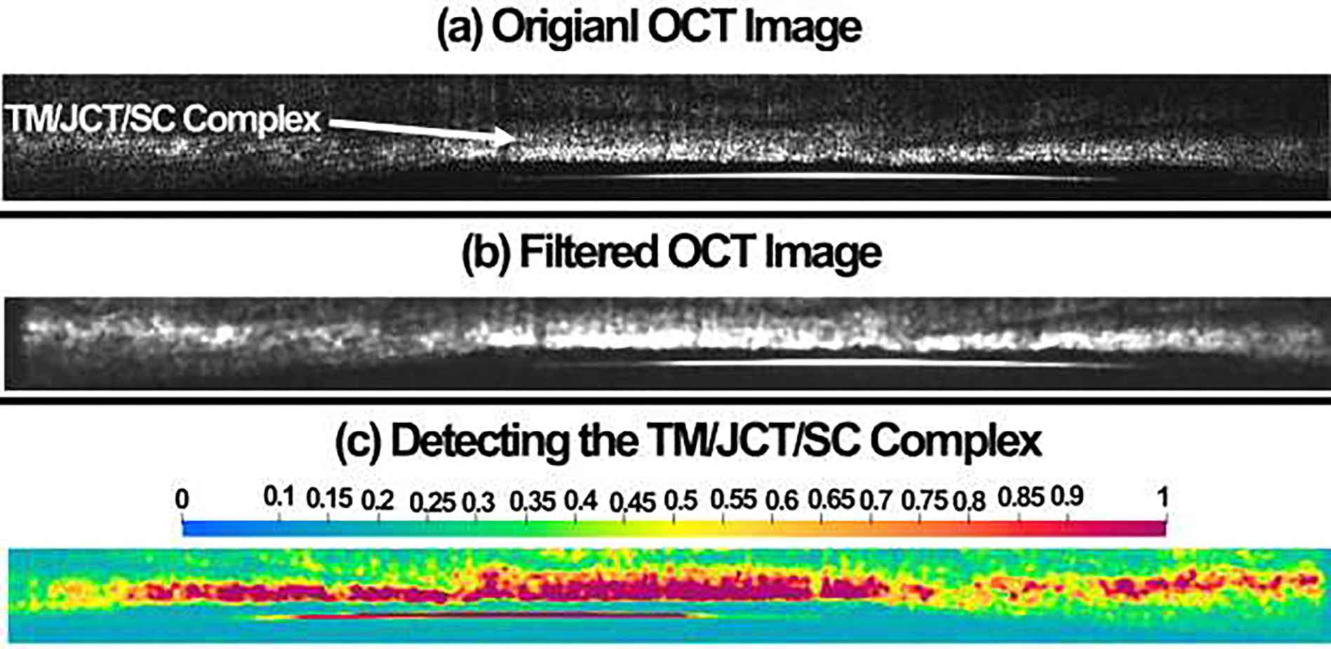
(a) Original OCT image was (b) median filtered for better pixel detection in the DVC code. (c) The DVC code detected the TM/JCT/SC complex based on the filtered data and the region of interest is defined with higher color bar magnitude.
3. Results
The optimized hyperviscoelastic material properties for the TM, JCT, and SC inner wall as well as the viscoelastic material properties for the collagen fibrils are reported in Table 2.
The experimental displacement in the SC inner wall, SC-JCT, JCT-TM, and TM nodes from the OCT images versus the inverse FE modeling data at four different cross-sections are displayed in Fig. 10.
Fig. 10.
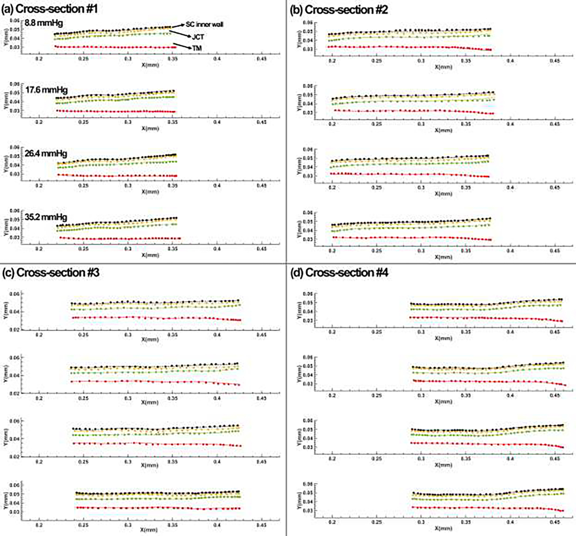
Comparison between the SC inner wall, SC-JCT, JCT-TM, and TM nodes from the OCT imaging data and the inverse finite element-optimization algorithm results at (a) cross-section #1, (b) cross-section #2, (c) cross-section #3, and (d) cross-section #4.
The DVC method calculated the resultant displacement, maximum shear strain, and 1st principal strain in the full stack of OCT images at the SC pressure of 0–17.6 mmHg and compared them to the FSI modeling results as shown in Fig. 11. Herein, to avoid having several figures with the same content, only the FSI and DVC data of pressure is provided.
Fig. 11.
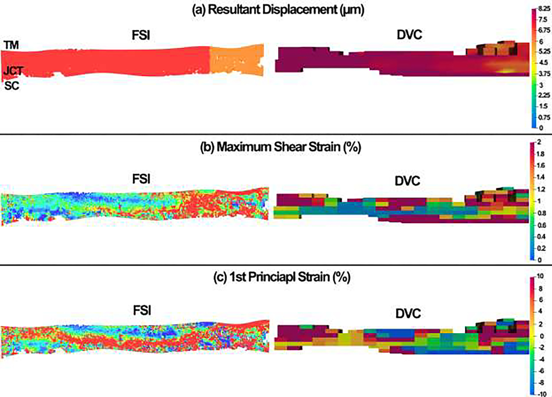
Comparison between the (a) resultant displacement, (b) maximum shear strain, and (c) 1st principal strain between the FSI simulation results and DVC data at the SC lumen pressure of 17.6mmHg.
The volumetric average resultant displacement, volumetric average maximum shear strain, and volumetric average 1st principal strain (tensile strain) in the FSI simulations and DVC analyses at different SC lumen pressures are summarized in Table 3.
Table 3.
Volumetric average resultant displacement, volumetric average maximum shear strain, and volumetric average 1st principal strain in the FSI simulation and DVC analysis at different SC lumen pressures.
| Parameters | Displacement (μm) | Maximum Shear Strain (%) 1s | t Principal Strain (%) |
|---|---|---|---|
|
| |||
| 8.8 mmHg | |||
|
| |||
| FSI | 2.75 | 0.55 | 2.02 |
| DVC | 2.81 | 0.49 | 2.08 |
|
| |||
| 17.6 mmHg | |||
|
| |||
| FSI | 5.75 | 1.05 | 4.16 |
| DVC | 5.85 | 1.12 | 4.15 |
|
| |||
| 26.4 mmHg | |||
|
| |||
| FSI | 8.02 | 1.69 | 6.77 |
| DVC | 8.10 | 1.85 | 6.95 |
|
| |||
| 35.2 mmHg 1C | |||
|
| |||
| FSI | 11.15 | 2.08 | 8.35 |
| DVC | 11.35 | 2.22 | 8.75 |
4. Discussion
The tensile elastic moduli for a human and porcine TM in the literature have been reported as orders of magnitude “MPa” [50, 54] larger compared to the reports that have used FE method and atomic force microscopy, where the moduli for the human TM were in the order of “kPa” [31, 40]. Both tensile mechanical measurement and atomic force microscopy are commonly used for biomechanical characterization of tissues. However, in the case of tensile testing, the tissue is typically pulled along the axis of the orientation of its fibers, while in atomic force microscopy, the tissue is locally poked or indented, which may not be aligned with the orientation of collagen and elastin fibers in a TM tissue [8]. The mechanical characterization of a tissue, including the calculation of its elastic modulus, is highly dependent on various test conditions such as sample preparation, tissue hydration, indenter geometry, and applied force or displacement rate. Similarly, atomic force microscopy testing may not accurately represent the mechanical behavior of the collagenous outflow tissues due to their anisotropic, viscoelastic, and large-deformation characteristics. In contrast, the inverse FE method can calculate tissue mechanical properties based on dynamic or static tissue motion while accounting for tissue complexities, loading, and boundary conditions. This approach provides a more realistic representation of tissue mechanical behavior at a lower cost, including labor and time. However, both methods have their own advantages and disadvantages that should be considered. The use of real-time OCT imaging may enhance the potential for the inverse FE-optimization algorithm to be utilized in early diagnosis of glaucoma based on the outflow tissues’ mechanical response to dynamic IOP. Ultimately, this approach may aid ophthalmologists in making clinical decisions and scientific studies of the effect of IOP-reducing drugs in glaucoma patients.
In this study, the inverse FE algorithm coupled with the unconstrained pattern search minimization algorithm was employed to calculate the hyperviscoelastic mechanical properties of the TM, JCT, and SC inner wall ECM with embedded viscoelastic collagen fibrils. The results showed good agreement with the experimental OCT nodal boundaries having the average mean percentage error of < 4.95% among all four cross-sections; this indicates the robustness and reliability of the proposed workflow in calculating the mechanical properties of the outflow tissues (Table 2 & Fig. 10). The TM showed the average shear modulus (μ) of 0.92 MPa, which was larger than the JCT (0.47 MPa) and SC inner wall (0.85 MPa) (Table 2). This is in good agreement with [35] where it is shown larger shear moduli for the TM compared to the JCT and SC. When it comes to the linear elastic mechanical properties of the conventional aqueous outflow tissues, there is a wide range of elastic moduli for the human TM in the literature (0.004 to 51.5 MPa [22]). Outflow is segmental with low- and high-flow regions [8] and it has been shown that the low-flow regions are mechanically stiffer compared to the high-flow regions [28, 99, 100]. While in this study, we have not done any pre-analysis to discern the low- and high-flow regions, and we have only used one quadrant of a normal human donor eye, larger shear moduli in the outflow tissues may implicitly telling us that the tested quadrant belonged to a low-flow region. In addition, the resultant shear moduli in the outflow tissues were found to be smaller compared to the sclera’s shear modulus that matches what most outflow scientists agree with. The average time-dependent shear modulus (G), however, was larger in the SC inner wall (97.65 MPa) compared to the TM (84.38 MPa) and JCT (56.30 MPa), implying a larger time-dependency in the biomechanical response of the SC inner wall. The collagen fibrils in the TM also showed a stiffer mechanical response compared to the JCT that may related to the larger deformation in the TM during distention compared to the JCT.
The optimized material properties that are summarized in Table 2 were assigned to the FSI model of the TM/JCT/SC complex (Fig. 7). The aqueous humor is flown from the SC lumen and passed through the SC inner wall pores to get into the JCT and then TM intratrabecular spaces. The maximum resultant displacement, maximum shear strain, and 1st principal (tensile) strain were then calculated in the FSI model and were compared to the DVC data at the SC lumen pressure of 0 to 17.6 mmHg (Fig. 11). A few things need to be carefully considered before interpreting the FSI and DVC results. First, the geometry of the TM/JCT/SC complex in the FSI model and DVC may not look exactly similar. This could be due to the difference in the initial geometry of the TM/JCT/SC complex at the SC lumen pressure of 0 mmHg that the FSI model was reconstructed. Two different algorithms were used to segment and detect the boundary of the TM/JCT/SC complex in the OCT images that may have affected the final geometry of the model at the SC lumen pressure of 17.6 mmHg. Second, the resultant color map, including the regions with larger and smaller displacement/strain as well as the size of the colored elements, may not look the same between the FSI and DVC data. This could be due to the initial geometry of the model at the SC lumen pressure of 0 mmHg as well as the accuracy of the algorithm that separated the outflow tissues from the interspersed aqueous humor. These could alter the intensity of the displacement/strain across the tissues. The cubic subsets of 5 pixels (=3.75-μm) per side and a node spacing of 15 pixels (=11.25-μm) were used in the DVC code for displacements calculation. However, in the FSI model, the element edge length was set to ~0.5μm and the simulation was conducted based on that assigned element edge length that could fairly affect the resultant color map and comparison across the FSI and DVC results. While this would require extra programming in the DVC code to reach smaller cubic subsets that matches the FSI model, herein, the resultant displacement in the FSI model is in good agreement with the DVC data illustrating larger displacement in the left lateral and center of the tissue complex while smaller in the right lateral (Fig. 11a). The maximum shear strain in the FSI model also matches with the DVC data indicating larger strains of ~2% and ~1.8% in the right lateral of the FS and DVC TM/JCT/SC complex, respectively (Fig. 11b). The 1st principal (tensile) strain also showed the same pattern in the FSI model compared to the DVC (Fig. 11c). When it comes to the volumetric average resultant displacement, volumetric average maximum shear strain, and volumetric average 1st principal strain in the FSI model, they are in good agreement with the DVC data (Table 3). This shows that the developed experimental-computational workflow is robust and reliable enough to calculate the hyperviscoelastic mechanical properties of the outflow tissues with embedded viscoelastic collagen fibrils. In future studies, the realistic physiologic condition of the aqueous outflow pathway can be modeled through aqueous humor entering the TM intratrabecular space from the anterior chamber, so we can calculate the resultant shear stresses across the outflow tissues and study the hydrodynamics of the aqueous humor with dynamic IOP.
The IOP elevation of 22 mmHg may cause up to 50% stretch in the cells of the outflow pathway [101]. The effects of the mechanical stress in the ECM of the outflow tissues as well as the resultant strain in the cells may all be considered as a potential pressure fluctuation mechanism that contributes to the regulation of the outflow facility and, consequently IOP [102]. Accurate calculations of stresses and strains in the outflow tissues depend on their mechanical properties. Given that these tissues experience large deformations and time-dependent biomechanical conditions, it is advisable to use their hyperviscoelastic properties in studying the biomechanics of the aqueous outflow pathway. Studies have demonstrated that the outflow tissues become stiffer with the progression of glaucoma [10, 22, 35, 103] and aqueous humor flow diminishes until it is eventually absent [3, 18, 104]. This suggests that the mechanical behavior of the conventional aqueous outflow tissues, which includes both hyperelastic and viscoelastic properties, may be impacted by the development of glaucoma. Thus, the hyperviscoelastic material model may allow us to not only capture the role of aging and glaucoma in the small- or large-deformation mechanical response of the outflow tissues but also the time-dependent shear modulus (G) of the tissues that depend on the rate of the IOP dynamic. Finally, the proposed FSI model that is validated versus the DVC data will be used in our future studies to calculate the biomechanical response of the outflow tissues and hydrodynamics of the aqueous humor across the outflow pathway with dynamic IOP from the anterior chamber.
4.1. Limitations
First, in a typical physiological scenario of the human conventional aqueous outflow pathway, the aqueous humor enters the outflow pathway from the anterior chamber, passing through the TM, JCT, and SC inner wall, and then exits through the SC pores into the SC lumen. However, in our organ culture preparation experiment, pressure is applied to the inner wall of the SC. In addition, the pressure in the SC lumen was elevated to 35.2 mmHg, but the physiological pressure in the SC lumen of a nonhuman primate is within 5.6–10.5 mmHg [105]. The high pressure of the aqueous humor used in our experiment enabled us to obtain the hyperelastic mechanical properties of the TM, JCT, and SC inner wall under large-deformation conditions, which would have been difficult to achieve with physiologic pressure load-boundaries applied from inside the eye. However, future experiments will involve cyclic positive and negative pressures applied to the SC lumen, which will provide a more realistic physiological load-boundary and validate the outflow tissues’ mechanical properties under both tension and compression, bringing us closer to a physiologic condition of the aqueous outflow pathway.
Second, it should be noted that the current study was limited to the analysis of a single healthy donor eye. Therefore, it is essential to investigate additional samples to represent the entire spectrum of geometries in individuals’ outflow tissues. The primary aim of this study was to establish an experimental-computational framework that enables us to pressurize the SC lumen, OCT image the TM/JCT/SC complex, and create a 3D microstructural FE model of the TM/JCT/SC complex from the same donor eye. In future investigations, a more extensive cohort of both healthy and glaucoma human eyes will be examined to cover the complete and diverse range of geometries in the outflow tissues.
Third, it is important to note that although we utilized a custom Matlab program and a glaucoma specialist to semi-automatically segment the boundaries of the TM, JCT, and SC inner wall, the accuracy of these segmented boundaries heavily relied on the resolution and contrast of the OCT images. While we took great care to avoid any errors in boundary recognition, it is possible that mistakes were made, which could have influenced the results of the inverse FE-optimization. Additionally, we assumed initial thicknesses of approximately 2μm and 5μm for the SC inner wall and JCT, respectively, which may vary in different cross-sections and quadrants of the eye. These assumptions could have affected the optimization algorithm and the resulting mechanical properties of these tissues. Moving forward, we plan to improve our OCT imaging setup with a wider bandwidth light source to increase image resolution and contrast, which will allow for more accurate boundary segmentation, particularly in the SC inner wall and JCT regions.
Fourth, in this study, it was not possible to simulate the segmental outflow due to the non-uniform flow in the 360° circumference of the TM structure, which is separated into low- and high-flow regions [106, 107]. However, in future studies, the low- and high-flow regions will be identified before conducting the experiments, and the material characterization will be performed on each tissue sample separately to accurately simulate the segmental outflow.
Fifth, the 3D FE model of the TM/JCT/SC complex was constructed based on green-light OCM data with a pixel size of 0.75μm. Although a higher resolution/contrast imaging data could improve the quality of the FE mesh, efforts are being made to develop an improved imaging system that can provide even higher quality FE mesh for more accurate FSI simulations in the future.
Sixth, the μm-sized pores in the SC were distributed at a density and size of 835 pores/mm2 [12] and 1.3 μm [77], respectively. The current model of the SC inner wall pores used in our study is not fully representative of the physiological geometry. However, in our future studies, we plan to improve the accuracy of our model by incorporating high-resolution SEM images of the SC inner wall. This will allow us to obtain a more realistic representation of the pore geometry and enable us to perform more accurate simulations of the aqueous humor flow through the outflow pathway.
Sixth, the modeling of the aqueous humor as a simple Newtonian fluid based on the rheological properties of a normal solution used in the organ culture perfusion setup may be a limitation of this study. In reality, the aqueous humor is a highly diluted solution that behaves rheologically as a Boger fluid, which exhibits similar properties to blood plasma [108]. To overcome this limitation, in future studies, we plan to include the complexity of the aqueous humor to better understand its rheological properties across the conventional outflow pathway.
Finally, although we assumed a uniform distribution of collagen fibrils in terms of length, diameter, stiffness, and distribution throughout the TM and JCT in our models, there is evidence to suggest that collagen fibrils closer to the anterior chamber are thicker than those nearer to the SC [57]. However, the quantitative information available on the density, morphology, and directionality of collagen fibrils in the outflow tissues is limited. In future studies, we aim to incorporate heterogeneous collagen fibril distributions into our modeling approach once more data becomes available. The final goal is to propose a faster and a more accurate image-to-modeling workflow that can be used in patients [109].
5. Conclusions
In this study, the hyperviscoelastic mechanical properties of the healthy aqueous outflow tissues with embedded viscoelastic collagen fibrils were characterized through dynamic SC pressurization and OCT imaging coupled with an inverse FE-optimization algorithm. The resulting 3D microstructural FE model of the TM/JCT/SC complex with embedded collagen fibrils and interspersed aqueous humor was subjected to a dynamic SC flow load boundary using the FSI method, and the resultant deformation/strain across the outflow tissues were compared to the DVC data. The study found that the TM showed larger hyperelastic and viscoelastic shear moduli compared to the JCT and SC. The accuracy and robustness of the experimental-computational workflow were validated against the DVC data. It is important to note that the hyperviscoelastic mechanical environment in the conventional aqueous outflow pathway is influenced by dynamic IOP fluctuations, which can have significant implications for ocular health. The development of a reliable and accurate experimental-computational workflow to calculate the mechanical properties of the outflow tissues is crucial for understanding the underlying mechanisms of glaucoma and improving diagnosis, treatment, and prevention of the disease. However, to fully realize the potential of this workflow, improvements in imaging technology are necessary to capture the dynamic motion of the TM/JCT/SC complex with higher resolution and frequency. This will enable the identification of biomechanical biomarkers for early detection and prediction of POAG severity and rate of progression, ultimately leading to better patient outcomes.
Fig. 8.
The pressure load-boundary applied on the SC inner wall.
Statement of significance.
While the human conventional aqueous outflow pathway is subjected to a large-deformation and time-dependent IOP load-boundary, we are not aware of any studies that have calculated the hyperviscoelastic mechanical properties of the outflow tissues with embedded viscoelastic collagen fibrils. A quadrant of the anterior segment of a normal humor donor eye was dynamically pressurized from the SC lumen with relatively large fluctuations. The TM/JCT/SC complex were OCT imaged and the mechanical properties of the tissues with embedded collagen fibrils were calculated using the inverse FE-optimization algorithm. The resultant displacement/strain in the FSI outflow model was validated versus the DVC data. The proposed experimental-computational workflow may significantly contribute to understanding of the effects of different drugs on the biomechanics of the conventional aqueous outflow pathway.
Acknowledgments
This work was supported in part by the NIH/NEI grants R01-EY030238, EY025721, EY026048, EY021800, EY003279, and EY008247, Lewis Rudin Glaucoma Prize and Research to Prevent Blindness Foundation (New York, New York) grant to the Casey Eye Institute.
Footnotes
Declaration of Competing Interest
The authors declare that they have no known competing financial interests or personal relationships that could have appeared to influence the work reported in this paper. All authors had access to the data and contributed to writing this manuscript.
Publisher's Disclaimer: This is a PDF file of an unedited manuscript that has been accepted for publication. As a service to our customers we are providing this early version of the manuscript. The manuscript will undergo copyediting, typesetting, and review of the resulting proof before it is published in its final form. Please note that during the production process errors may be discovered which could affect the content, and all legal disclaimers that apply to the journal pertain.
Data availability
The raw/processed data required to reproduce these findings cannot be shared at this time as the data is part of an ongoing study.
References
- [1].Dvorak-Theobald G, Kirk HQ, Aqueous pathways in some cases of glaucoma, Trans Am Ophthalmol Soc 53 (1955) 301. [PMC free article] [PubMed] [Google Scholar]
- [2].Johnstone MA, The aqueous outflow system as a mechanical pump: evidence from examination of tissue and aqueous movement in human and non-human primates, J Glaucoma 13(5) (2004) 421–38. [DOI] [PubMed] [Google Scholar]
- [3].Johnstone M, Jamil A, Martin E, Aqueous veins and open angle glaucoma, The Glaucoma Book, Springer; 2010, pp. 65–78. [Google Scholar]
- [4].Johnstone MA, Intraocular pressure regulation: findings of pulse-dependent trabecular meshwork motion lead to unifying concepts of intraocular pressure homeostasis, Mary Ann Liebert, Inc. 140 Huguenot Street, 3rd Floor New Rochelle, NY 10801 USA, 2014. [DOI] [PMC free article] [PubMed] [Google Scholar]
- [5].Johnstone M, Xin C, Tan J, Martin E, Wen J, Wang RK, Aqueous outflow regulation-21st century concepts, Prog Retin Eye Res (2020) 100917. [DOI] [PMC free article] [PubMed] [Google Scholar]
- [6].Johnson MC, Kamm RD, The role of Schlemm’s canal in aqueous outflow from the human eye, Invest Ophthalmol Vis Sci 24(3) (1983) 320–5. [PubMed] [Google Scholar]
- [7].Stamer WD, Braakman ST, Zhou EH, Ethier CR, Fredberg JJ, Overby DR, Johnson M, Biomechanics of Schlemm’s canal endothelium and intraocular pressure reduction, Prog Retin Eye Res 44 (2015) 86–98. [DOI] [PMC free article] [PubMed] [Google Scholar]
- [8].Acott TS, Vranka JA, Keller KE, Raghunathan V, Kelley MJ, Normal and glaucomatous outflow regulation, Prog Retin Eye Res 82 (2021) 100897. [DOI] [PMC free article] [PubMed] [Google Scholar]
- [9].Karimi A, Razaghi R, Rahmati SM, Downs JC, Acott TS, Wang RK, Johnstone M, Modeling the biomechanics of the conventional aqueous outflow pathway microstructure in the human eye, Comput Methods Programs Biomed 221 (2022) 106922. [DOI] [PMC free article] [PubMed] [Google Scholar]
- [10].Karimi A, Rahmati SM, Razaghi R, Crawford Downs J, Acott TS, Wang RK, Johnstone M, Biomechanics of human trabecular meshwork in healthy and glaucoma eyes via dynamic Schlemm’s canal pressurization, Comput Methods Programs Biomed 221 (2022) 106921. [DOI] [PMC free article] [PubMed] [Google Scholar]
- [11].Johnstone MA, Grant WG, Pressure-dependent changes in structures of the aqueous outfiow system of human and monkey eyes, Am J Ophthalmol 75(3) (1973) 365–83. [DOI] [PubMed] [Google Scholar]
- [12].Johnson M, Chan D, Read AT, Christensen C, Sit A, Ethier CR, The pore density in the inner wall endothelium of Schlemm’s canal of glaucomatous eyes, Invest Ophthalmol Vis Sci 43(9) (2002) 2950–5. [PubMed] [Google Scholar]
- [13].Goel M, Picciani RG, Lee RK, Bhattacharya SK, Aqueous humor dynamics: a review, Open Ophthalmol J 4 (2010) 52–9. [DOI] [PMC free article] [PubMed] [Google Scholar]
- [14].Acott TS, Kelley MJ, Keller KE, Vranka JA, Abu-Hassan DW, Li X, Aga M, Bradley JM, Intraocular pressure homeostasis: maintaining balance in a high-pressure environment, J Ocul Pharmacol Ther 30(2–3) (2014) 94–101. [DOI] [PMC free article] [PubMed] [Google Scholar]
- [15].Abu-Hassan DW, Li X, Ryan EI, Acott TS, Kelley MJ, Induced pluripotent stem cells restore function in a human cell loss model of open-angle glaucoma, Stem Cells 33(3) (2015) 751–61. [DOI] [PMC free article] [PubMed] [Google Scholar]
- [16].Bradley JM, Kelley MJ, Zhu X, Anderssohn AM, Alexander JP, Acott TS, Effects of mechanical stretching on trabecular matrix metalloproteinases, Invest Ophthalmol Vis Sci 42(7) (2001) 1505–13. [PubMed] [Google Scholar]
- [17].Overby DR, Stamer WD, Johnson M, The changing paradigm of outflow resistance generation: towards synergistic models of the JCT and inner wall endothelium, Exp Eye Res 88(4) (2009) 656–70. [DOI] [PMC free article] [PubMed] [Google Scholar]
- [18].Gao K, Song S, Johnstone MA, Zhang Q, Xu J, Zhang X, Wang RK, Wen JC, Reduced Pulsatile Trabecular Meshwork Motion in Eyes With Primary Open Angle Glaucoma Using Phase-Sensitive Optical Coherence Tomography, Invest Ophthalmol Vis Sci 61(14) (2020) 21. [DOI] [PMC free article] [PubMed] [Google Scholar]
- [19].Xin C, Wang XF, Wang NL, Wang RK, Johnstone M, Trabecular Meshwork Motion Profile from Pulsatile Pressure Transients: A New Platform to Simulate Transitory Responses in Humans and Nonhuman Primates, Appl Sci-Basel 12(1) (2022) 11. [Google Scholar]
- [20].Li P, Reif R, Zhi Z, Martin E, Shen TT, Johnstone M, Wang RK, Phase-sensitive optical coherence tomography characterization of pulse-induced trabecular meshwork displacement in ex vivo nonhuman primate eyes, J Biomed Opt 17(7) (2012) 076026. [DOI] [PubMed] [Google Scholar]
- [21].Li P, Shen TT, Johnstone M, Wang RK, Pulsatile motion of the trabecular meshwork in healthy human subjects quantified by phase-sensitive optical coherence tomography, Biomed. Opt. Express 4(10) (2013) 2051–65. [DOI] [PMC free article] [PubMed] [Google Scholar]
- [22].Wang K, Read AT, Sulchek T, Ethier CR, Trabecular meshwork stiffness in glaucoma, Exp Eye Res 158 (2017) 3–12. [DOI] [PMC free article] [PubMed] [Google Scholar]
- [23].Xin C, Song S, Johnstone M, Wang N, Wang RK, Quantification of Pulse-Dependent Trabecular Meshwork Motion in Normal Humans Using Phase-Sensitive OCT Invest Ophthalmol Vis Sci 59(8) (2018) 3675–3681. [DOI] [PMC free article] [PubMed] [Google Scholar]
- [24].Gao K, Song SZ, Johnstone MA, Wang RKK, Wen JC, Trabecular Meshwork Motion in Normal Compared with Glaucoma Eyes, Invest Ophthalmol Vis Sci 60(9) (2019) 4824–4824. [Google Scholar]
- [25].Du R, Xin C, Xu J, Hu J, Wang H, Wang N, Johnstone M, Pulsatile Trabecular Meshwork Motion: An Indicator of Intraocular Pressure Control in Primary Open-Angle Glaucoma, J Clin Med 11(10) (2022) 2696. [DOI] [PMC free article] [PubMed] [Google Scholar]
- [26].Turner DC, Edmiston AM, Zohner YE, Byrne KJ, Seigfreid WP, Girkin CA, Morris JS, Downs JC, Transient Intraocular Pressure Fluctuations: Source, Magnitude, Frequency, and Associated Mechanical Energy, Invest Ophthalmol Vis Sci 60(7) (2019) 2572–2582. [DOI] [PMC free article] [PubMed] [Google Scholar]
- [27].Karimi A, Razaghi R, Rahmati SM, Downs JC, Acott TS, Kelley MJ, Wang RK, Johnstone M, The Effect of Intraocular Pressure Load Boundary on the Biomechanics of the Human Conventional Aqueous Outflow Pathway, Bioengineering (Basel) 9(11) (2022) 672–689. [DOI] [PMC free article] [PubMed] [Google Scholar]
- [28].Vranka JA, Staverosky JA, Reddy AP, Wilmarth PA, David LL, Acott TS, Russell P, Raghunathan VK, Biomechanical Rigidity and Quantitative Proteomics Analysis of Segmental Regions of the Trabecular Meshwork at Physiologic and Elevated Pressures, Invest Ophthalmol Vis Sci 59(1) (2018) 246–259. [DOI] [PMC free article] [PubMed] [Google Scholar]
- [29].Silver FH, Seehra GP, Freeman JW, DeVore D, Viscoelastic properties of young and old human dermis: A proposed molecular mechanism for elastic energy storage in collagen and elastin, J Appl Polym Sci 86(8) (2002) 1978–1985. [Google Scholar]
- [30].Ryan AJ, O’Brien FJ, Insoluble elastin reduces collagen scaffold stiffness, improves viscoelastic properties, and induces a contractile phenotype in smooth muscle cells, Biomaterials 73 (2015) 296–307. [DOI] [PubMed] [Google Scholar]
- [31].Last JA, Pan T, Ding Y, Reilly CM, Keller K, Acott TS, Fautsch MP, Murphy CJ, Russell P, Elastic modulus determination of normal and glaucomatous human trabecular meshwork, Invest Ophthalmol Vis Sci 52(5) (2011) 2147–52. [DOI] [PMC free article] [PubMed] [Google Scholar]
- [32].Russell P, Johnson M, Elastic Modulus Determination of Normal and Glaucomatous Human Trabecular Meshwork Invest Ophthalmol Vis Sci 53(1) (2012) 117–117. [DOI] [PubMed] [Google Scholar]
- [33].Vahabikashi A, Gelman A, Dong B, Gong L, Cha EDK, Schimmel M, Tamm ER, Perkumas K, Stamer WD, Sun C, Zhang HF, Gong H, Johnson M, Increased stiffness and flow resistance of the inner wall of Schlemm’s canal in glaucomatous human eyes, Proc Natl Acad Sci U S A 116(52) (2019) 26555–26563. [DOI] [PMC free article] [PubMed] [Google Scholar]
- [34].Pant AD, Kagemann L, Schuman JS, Sigal IA, Amini R, An imaged-based inverse finite element method to determine in-vivo mechanical properties of the human trabecular meshwork, J Model Ophthalmol 1(3) (2017) 100–111. [PMC free article] [PubMed] [Google Scholar]
- [35].Karimi A, Razaghi R, Padilla S, Rahmati SM, Downs JC, Acott TS, Kelley MJ, Wang RK, Johnstone M, Viscoelastic Biomechanical Properties of the Conventional Aqueous Outflow Pathway Tissues in Healthy and Glaucoma Human Eyes, J Clin Med 11(20) (2022) 6049. [DOI] [PMC free article] [PubMed] [Google Scholar]
- [36].Khan S, Neuhaus K, Thaware O, Ni S, Ju MJ, Redd T, Huang D, Jian Y, Corneal imaging with blue-light optical coherence microscopy, Biomed. Opt. Express 13(9) (2022) 5004–5014. [DOI] [PMC free article] [PubMed] [Google Scholar]
- [37].Karimi A, Rahmati SM, Razaghi R, Girkin CA, Crawford Downs J, Finite element modeling of the complex anisotropic mechanical behavior of the human sclera and pia mater, Comput Methods Programs Biomed 215(3) (2022) 106618. [DOI] [PMC free article] [PubMed] [Google Scholar]
- [38].Tudisco E, Ando E, Cailletaud R, Hall SA, TomoWarp2: A local digital volume correlation code, Softwarex 6 (2017) 267–270. [Google Scholar]
- [39].Acott TS, Kingsley PD, Samples JR, Van Buskirk EM, Human trabecular meshwork organ culture: morphology and glycosaminoglycan synthesis, Invest Ophthalmol Vis Sci 29(1) (1988) 90–100. [PubMed] [Google Scholar]
- [40].Wang K, Johnstone MA, Xin C, Song S, Padilla S, Vranka JA, Acott TS, Zhou K, Schwaner SA, Wang RK, Sulchek T, Ethier CR, Estimating Human Trabecular Meshwork Stiffness by Numerical Modeling and Advanced OCT Imaging, Invest Ophthalmol Vis Sci 58(11) (2017) 4809–4817. [DOI] [PMC free article] [PubMed] [Google Scholar]
- [41].Hariri S, Johnstone M, Jiang Y, Padilla S, Zhou Z, Reif R, Wang RK, Platform to investigate aqueous outflow system structure and pressure-dependent motion using high-resolution spectral domain optical coherence tomography, J Biomed Opt 19(10) (2014) 106013. [DOI] [PMC free article] [PubMed] [Google Scholar]
- [42].Nguyen TP, Ni S, Ostmo S, Rajagopalan A, Coyner AS, Woodward M, Chiang MF, Jia Y, Huang D, Campbell JP, Jian Y, Association of Optical Coherence Tomography-Measured Fibrovascular Ridge Thickness and Clinical Disease Stage in Retinopathy of Prematurity, JAMA Ophthalmol 140(11) (2022) 1121–7. [DOI] [PMC free article] [PubMed] [Google Scholar]
- [43].Jian YF, Wong K, Sarunic MV, Graphics processing unit accelerated optical coherence tomography processing at megahertz axial scan rate and high resolution video rate volumetric rendering, J Biomed Optics 18(2) (2013) 026002. [DOI] [PubMed] [Google Scholar]
- [44].Camino A, Ng R, Huang J, Guo Y, Ni S, Jia Y, Huang D, Jian Y, Depth-resolved optimization of a real-time sensorless adaptive optics optical coherence tomography, Opt Lett 45(9) (2020) 2612–2615. [DOI] [PubMed] [Google Scholar]
- [45].Nagy AP, 1 Fundamentals of nonlinear elasticity, (2020).
- [46].Crisfield M, Galvanetto U, Jelenić G, Dynamics of 3-D co-rotational beams, Comput Mech 20(6) (1997) 507–519. [Google Scholar]
- [47].Manual L-DT, Livermore software technology corporation, Livermore, CA: 199 (1998). [Google Scholar]
- [48].Herrmann L, A numerical procedure for viscoelastic stress analysis, Seventh Meeting of ICRPG Mechanical Behavior Working Group, Orlando, FL, 1968, 1968. [Google Scholar]
- [49].LS-DYNA, LS-DYNA User Manual Volume 2 and Theory Manual, Version R13.
- [50].Camras LJ, Stamer WD, Epstein D, Gonzalez P, Yuan F, Differential effects of trabecular meshwork stiffness on outflow facility in normal human and porcine eyes, Invest Ophthalmol Vis Sci 53(9) (2012) 5242–50. [DOI] [PubMed] [Google Scholar]
- [51].Abdolkarimzadeh F, Ashory MR, Ghasemi-Ghalebahman A, Karimi A, Inverse dynamic finite element-optimization modeling of the brain tumor mass-effect using a variable pressure boundary, Comput Methods Programs Biomed 212 (2021) 106476. [DOI] [PubMed] [Google Scholar]
- [52].Rahmati SM, Razaghi R, Karimi A, Biomechanics of the keratoconic cornea: Theory, segmentation, pressure distribution, and coupled FE-optimization algorithm, J Mech Behav Biomed Mater 113 (2021) 104155. [DOI] [PubMed] [Google Scholar]
- [53].Schmidt DA, Shi C, Berry RA, Honig ML, Utschick W, Minimum mean squared error interference alignment, 2009 Conference Record of the Forty-Third Asilomar Conference on Signals, Systems and Computers, IEEE, 2009, pp. 1106–1110. [Google Scholar]
- [54].Camras LJ, Stamer WD, Epstein D, Gonzalez P, Yuan F, Circumferential tensile stiffness of glaucomatous trabecular meshwork, Invest Ophthalmol Vis Sci 55(2) (2014) 814–23. [DOI] [PubMed] [Google Scholar]
- [55].Horová I, Kolacek J, Zelinka J, Kernel Smoothing in MATLAB: theory and practice of kernel smoothing, World scientific; 2012. [Google Scholar]
- [56].Karimi A, Rahmati SM, Grytz RG, Girkin CA, Downs JC, Modeling the biomechanics of the lamina cribrosa microstructure in the human eye, Acta Biomater 134 (2021) 357–378. [DOI] [PMC free article] [PubMed] [Google Scholar]
- [57].Flocks M, The anatomy of the trabecular meshwork as seen in tangential section, AMA Arch Ophthalmol 56(5) (1956) 708–718. [DOI] [PubMed] [Google Scholar]
- [58].Hogan MJ, Histology of the human eye, An atlas and textbook (1971). [Google Scholar]
- [59].Umihira J, Nagata S, Nohara M, Hanai T, Usuda N, Segawa K, Localization of elastin in the normal and glaucomatous human trabecular meshwork, Invest Ophthalmol Vis Sci 35(2) (1994) 486–94. [PubMed] [Google Scholar]
- [60].Morishige N, Petroll WM, Nishida T, Kenney MC, Jester JV, Noninvasive corneal stromal collagen imaging using two-photon-generated second-harmonic signals, J Cataract Refract Surg 32(11) (2006) 1784–91. [DOI] [PMC free article] [PubMed] [Google Scholar]
- [61].Ammar DA, Lei TC, Gibson EA, Kahook MY, Two-photon imaging of the trabecular meshwork, Mol Vis 16 (2010) 935–44. [PMC free article] [PubMed] [Google Scholar]
- [62].Johnstone MA, Hariri S, Jiang Y, Padilla S, Zhou ZH, Wang RKK, OCT Imaging Shows Collector Channels Rapidly Open & Close with Pressure Changes: A Mechanism Regulating Control of Distal Resistance?, Invest Ophthalmol Vis Sci 56(7) (2015) 3539–3539. [Google Scholar]
- [63].Park CY, Lee JK, Kahook MY, Schultz JS, Zhang C, Chuck RS, Revisiting ciliary muscle tendons and their connections with the trabecular meshwork by two photon excitation microscopic imaging, Invest Ophthalmol Vis Sci 57(3) (2016) 1096–1105. [DOI] [PubMed] [Google Scholar]
- [64].Belytschko T, Lu YY, Gu L, Element-free Galerkin methods, Int J Numer Methods Eng 37(2) (1994) 229–256. [Google Scholar]
- [65].Chen H, An introduction to* CONSTRAINED_BEAM_IN_SOLID, FEA Information (2016) 79–83. [Google Scholar]
- [66].Ma K, Farajzadeh R, Lopez-Salinas JL, Miller CA, Biswal SL, Hirasaki GJ, Non-uniqueness, Numerical Artifacts, and Parameter Sensitivity in Simulating Steady-State and Transient Foam Flow Through Porous Media, Transport in Porous Media 102(3) (2014) 325–348. [Google Scholar]
- [67].Chiandussi G, Codegone M, Ferrero S, Varesio FE, Comparison of multi-objective optimization methodologies for engineering applications, Computers & Mathematics with Applications 63(5) (2012) 912–942. [Google Scholar]
- [68].Goffe WL, Ferrier GD, Rogers J, Global Optimization of Statistical Functions with Simulated Annealing, J Econometr 60(1–2) (1994) 65–99. [Google Scholar]
- [69].Abdollahi H, Tauler R, Uniqueness and rotation ambiguities in Multivariate Curve Resolution methods, Chemometrics and Intelligent Laboratory Systems 108(2) (2011) 100–111. [Google Scholar]
- [70].Fang Q, Boas DA, Tetrahedral mesh generation from volumetric binary and grayscale images, 2009 IEEE international symposium on biomedical imaging: from nano to macro, IEEE, 2009, pp. 1142–1145. [Google Scholar]
- [71].Tran AP, Yan S, Fang Q, Improving model-based functional near-infrared spectroscopy analysis using mesh-based anatomical and light-transport models, Neurophotonics 7(1) (2020) 015008–015008. [DOI] [PMC free article] [PubMed] [Google Scholar]
- [72].Rineau L, Yvinec M, 3D surface mesh generation, CGAL user and reference manual 4(1) (2012). [Google Scholar]
- [73].Attene M, Falcidieno B, Remesh: An interactive environment to edit and repair triangle meshes, IEEE International Conference on Shape Modeling and Applications 2006 (SMI’06), IEEE, 2006, pp. 41–41. [Google Scholar]
- [74].Karimi A, Razaghi R, Rahmati SM, Girkin CA, Downs JC, Relative Contributions of Intraocular and Cerebrospinal Fluid Pressures to the Biomechanics of the Lamina Cribrosa and Laminar Neural Tissues, Invest Ophthalmol Vis Sci 63(11) (2022) 14. [DOI] [PMC free article] [PubMed] [Google Scholar]
- [75].Ten Hulzen RD, Johnson DH, Effect of fixation pressure on juxtacanalicular tissue and Schlemm’s canal, Invest Ophthalmol Vis Sci 37(1) (1996) 114–24. [PubMed] [Google Scholar]
- [76].Overby D, Gong H, Qiu G, Freddo TF, Johnson M, The mechanism of increasing outflow facility during washout in the bovine eye, Invest Ophthalmol Vis Sci 43(11) (2002) 3455–64. [PubMed] [Google Scholar]
- [77].Ethier CR, Coloma FM, Sit AJ, Johnson M, Two pore types in the inner-wall endothelium of Schlemm’s canal, Invest Ophthalmol Vis Sci 39(11) (1998) 2041–8. [PubMed] [Google Scholar]
- [78].Anderson DR, The development of the trabecular meshwork and its abnormality in primary infantile glaucoma, Trans Am Ophthalmol Soc 79 (1981) 458–85. [PMC free article] [PubMed] [Google Scholar]
- [79].Rehnberg M, Ammitzboll T, Tengroth B, Collagen distribution in the lamina cribrosa and the trabecular meshwork of the human eye, BrJ Ophthalmol 71(12) (1987) 886–92. [DOI] [PMC free article] [PubMed] [Google Scholar]
- [80].Vranka JA, Kelley MJ, Acott TS, Keller KE, Extracellular matrix in the trabecular meshwork: intraocular pressure regulation and dysregulation in glaucoma, Exp Eye Res 133 (2015) 112–25. [DOI] [PMC free article] [PubMed] [Google Scholar]
- [81].Bill A, Svedbergh B, Scanning electron microscopic studies of the trabecular meshwork and the canal of Schlemm--an attempt to localize the main resistance to outflow of aqueous humor in man, Acta Ophthalmol (Copenh) 50(3) (1972) 295–320. [DOI] [PubMed] [Google Scholar]
- [82].Allingham RR, Dekater AW, Ethier CR, Anderson PJ, Hertzmark E, Epstein DL, The Relationship between Pore Density and Outflow Facility in Human Eyes, Invest Ophthalmol Vis Sci 33(5) (1992) 1661–1669. [PubMed] [Google Scholar]
- [83].Perkins TW, Alvarado JA, Polansky JR, Stilwell L, Maglio M, Juster R, Trabecular meshwork cells grown on filters. Conductivity and cytochalasin effects, Invest Ophthalmol Vis Sci 29(12) (1988) 1836–46. [PubMed] [Google Scholar]
- [84].Ethier CR, Kamm RD, Palaszewski BA, Johnson MC, Richardson TM, Calculations of flow resistance in the juxtacanalicular meshwork, Invest Ophthalmol Vis Sci 27(12) (1986) 1741–50. [PubMed] [Google Scholar]
- [85].Johnson M, What controls aqueous humour outflow resistance?, Exp Eye Res 82(4) (2006) 545–557. [DOI] [PMC free article] [PubMed] [Google Scholar]
- [86].Souli M, ALE incompressible fluid in LS-DYNA, Proceedings of the 11th International LS-DYNA Conference. Detroit, MI, USA, 2010, pp. 29–36. [Google Scholar]
- [87].Aquelet N, Souli M, ALE Incompressible Fluid in LS-DYNA®, FSI/ALE 21 (2012) [Google Scholar]
- [88].Peery JS, Carroll DE, Multi-Material ALE methods in unstructured grids, Comput Methods Appl Mech Eng 187(3–4) (2000) 591–619. [Google Scholar]
- [89].Aquelet N, ALE adaptive mesh refinement in LS-Dyna, 12th International LS-DYNA Users Conference, 2012. [Google Scholar]
- [90].Razaghi R, Biglari H, Karimi A, Risk of rupture of the cerebral aneurysm in relation to traumatic brain injury using a patient-specific fluid-structure interaction model, Comput Methods Programs Biomed 176 (2019) 9–16. [DOI] [PubMed] [Google Scholar]
- [91].Vass C, Hirn C, Unger E, Mayr W, Georgopoulos M, Rainer G, Richter-Maksch S, Human aqueous humor viscosity in cataract, primary open angle glaucoma and pseudoexfoliation syndrome., Invest Ophthalmol Vis Sci 45(13) (2004) U564–U564. [Google Scholar]
- [92].Hughes TJ, Liu WK, Zimmermann TK, Lagrangian-Eulerian finite element formulation for incompressible viscous flows, Comput Methods Appl Mech Eng 29(3) (1981) 329–349. [Google Scholar]
- [93].Souli M, ALE incompressible fluid in LS-DYNA, Proceedings of the 11th International LS-DYNA Conference, Detroit, MI, USA, 2010, pp. 6–8. [Google Scholar]
- [94].Souli M, Ouahsine A, Lewin L, ALE formulation for fluid-structure interaction problems, Comput Methods Appl Mech Eng 190(5–7) (2000) 659–675. [Google Scholar]
- [95].Murray YD, Users manual for LS-DYNA concrete material model 159, United States. Federal Highway Administration. Office of Research, 2007. [Google Scholar]
- [96].Karimi A, Navidbakhsh M, Razaghi R, Haghpanahi M, A computational fluid-structure interaction model for plaque vulnerability assessment in atherosclerotic human coronary arteries, J Appl Phys 115(14) (2014) 144702. [Google Scholar]
- [97].Karimi A, Navidbakhsh M, Razaghi R, Plaque and arterial vulnerability investigation in a three-layer atherosclerotic human coronary artery using computational fluid-structure interaction method, J Appl Phys 116(6) (2014) 064701. [Google Scholar]
- [98].Razaghi R, Karimi A, Rahmani S, Navidbakhsh M, A computational fluid-structure interaction model of the blood flow in the healthy and varicose saphenous vein, Vascular 24(3) (2016) 254–63. [DOI] [PubMed] [Google Scholar]
- [99].Vranka JA, Raghunathan V, Russell P, Keller KE, Reddy A, Wilmarth P, Klimek J, David LL, Acott TS, Biomechanical Rigidity and Proteomics Analyses of Segmental Outflow Regions of the Trabecular Meshwork at Physiologic and Elevated Pressures, Invest Ophthalmol Vis Sci 57(12) (2016) 4702–4702. [DOI] [PMC free article] [PubMed] [Google Scholar]
- [100].Keller KE, Peters DM, Pathogenesis of glaucoma: Extracellular matrix dysfunction in the trabecular meshwork-A review, Clin Exp Ophthalmol 50(2) (2022) 163–182. [DOI] [PMC free article] [PubMed] [Google Scholar]
- [101].Grierson I, Lee WR, Light microscopic quantitation of the endothelial vacuoles in Schlemm’s canal, Am J Ophthalmol 84(2) (1977) 234–46. [DOI] [PubMed] [Google Scholar]
- [102].Liton PB, Gonzalez P, Stress response of the trabecular meshwork, J Glaucoma 17(5) (2008) 378–85. [DOI] [PMC free article] [PubMed] [Google Scholar]
- [103].Raghunathan VK, Benoit J, Kasetti R, Zode G, Salemi M, Phinney BS, Keller KE, Staverosky JA, Murphy CJ, Acott T, Vranka J, Glaucomatous cell derived matrices differentially modulate non-glaucomatous trabecular meshwork cellular behavior, Acta Biomater 71 (2018) 444–459. [DOI] [PMC free article] [PubMed] [Google Scholar]
- [104].Ascher KW, The Aqueous Veins: Biomicroscopic Study of the Aqueous Humor Elimination, Thomas 1961. [Google Scholar]
- [105].Maepea O, Bill A, Pressures in the juxtacanalicular tissue and Schlemm’s canal in monkeys, Exp Eye Res 54(6) (1992) 879–83. [DOI] [PubMed] [Google Scholar]
- [106].Stamer WD, Acott TS, Current understanding of conventional outflow dysfunction in glaucoma, Curr Opin Ophthalmol 23(2) (2012) 135–43. [DOI] [PMC free article] [PubMed] [Google Scholar]
- [107].Carreon T, van der Merwe E, Fellman RL, Johnstone M, Bhattacharya SK, Aqueous outflow - A continuum from trabecular meshwork to episcleral veins, Prog Retin Eye Res 57 (2017) 108–133. [DOI] [PMC free article] [PubMed] [Google Scholar]
- [108].Varchanis S, Dimakopoulos Y, Wagner C, Tsamopoulos J, How viscoelastic is human blood plasma?, Soft Matter 14(21) (2018) 4238–4251. [DOI] [PubMed] [Google Scholar]
- [109].Karimi A, Crouch DJ, Razaghi R, Downs JC, Acott TS, Kelley MJ, Behnsen JG, Bosworth LA, Sheridan CM, Morphological and Biomechanical Analyses of the Human Healthy and Glaucomatous Aqueous Outflow Pathway: Imaging-to-Modeling, Comput Methods Programs Biomed (2023) 107485. [DOI] [PMC free article] [PubMed] [Google Scholar]
- [110].Sherwood JM, Stamer WD, Overby DR, A model of the oscillatory mechanical forces in the conventional outflow pathway, J R Soc Interface 16(150) (2019) 20180652. [DOI] [PMC free article] [PubMed] [Google Scholar]
- [111].Johnstone M, Xin C, Acott T, Vranka J, Wen J, Martin E, Wang RK, Valve-Like Outflow System Behavior With Motion Slowing in Glaucoma Eyes: Findings Using a Minimally Invasive Glaucoma Surgery–MIGS-Like Platform and Optical Coherence Tomography Imaging, Front Med (2022) 1138. [DOI] [PMC free article] [PubMed] [Google Scholar]
Associated Data
This section collects any data citations, data availability statements, or supplementary materials included in this article.
Data Availability Statement
The raw/processed data required to reproduce these findings cannot be shared at this time as the data is part of an ongoing study.