. 2023 May 17;12:e81774. doi: 10.7554/eLife.81774

Figure 3. The effect of spontaneous state fluctuations on accuracy is outcome dependent.

(A) Coefficients of a generalized linear mixed model (GLMM) fit to the mice’s choice accuracy in valid trials. Accuracy is affected by the strength of evidence, the point during the session and the outcome of the previous trial, but none of the four signals computed during the baseline explain accuracy. (B) Mean difference in accuracy after errors minus after corrects in each of the recording sessions. Triangle, median across sessions. (C) GLMM fit to accuracy computed separately after error trials. On the right, we show the distribution of a single coefficient capturing trial-to-trial fluctuations in desynchronization and firing rate simultaneously (see text). (D) Psychometric function (logistic fit, Methods) of aggregate data across sessions separately for trials with favorable (SynchI(z)<0 and FRI(z)>0) and unfavorable (SynchI(z)>0 and FRI(z)<0) baseline states after a error trials. (E, F) Same as (C, D) but for choices after a correct trial. Note that, based on the results in (E), the favorable state after a correct trial is SynchI(z)>0 and FRI(z)>0. (G) Schematic illustration of possible relationships between outcome, baseline cortical state and accuracy. Left, the association between state and accuracy is spurious and results from a common effect of response outcome on these two variables. Middle, epoch hypothesis (see text). An unmeasured variable with a timescale of several trials mediates both the effect of state on accuracy and the prevalence of errors. Right, response outcome gates the effect of state fluctuations (errors open the gate) on choice accuracy. (H, I) Same as (C, E) but conditioned on the outcome of the next, rather than the previous trial.
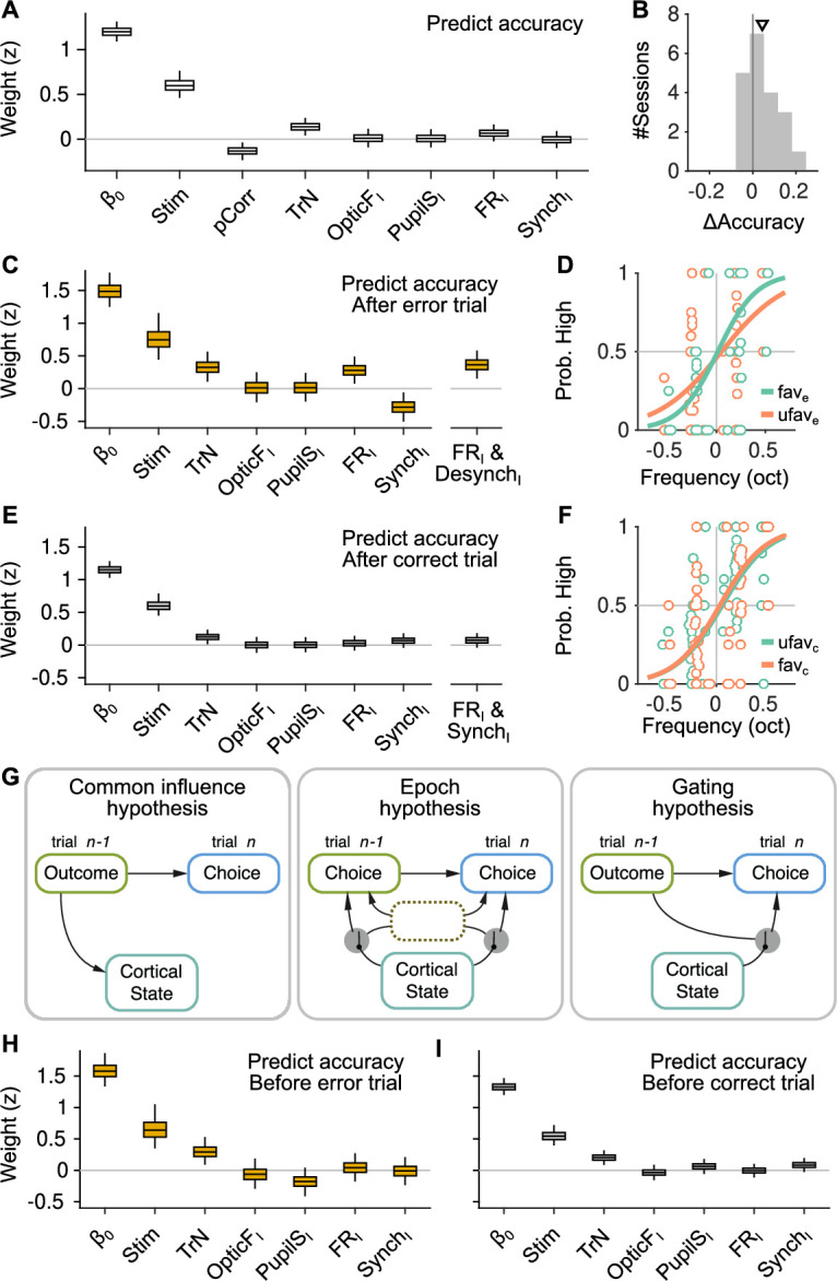
Figure 3.

Figure 3—figure supplement 1. Robustness of the association between brain state and accuracy.

Figure 3—figure supplement 1.

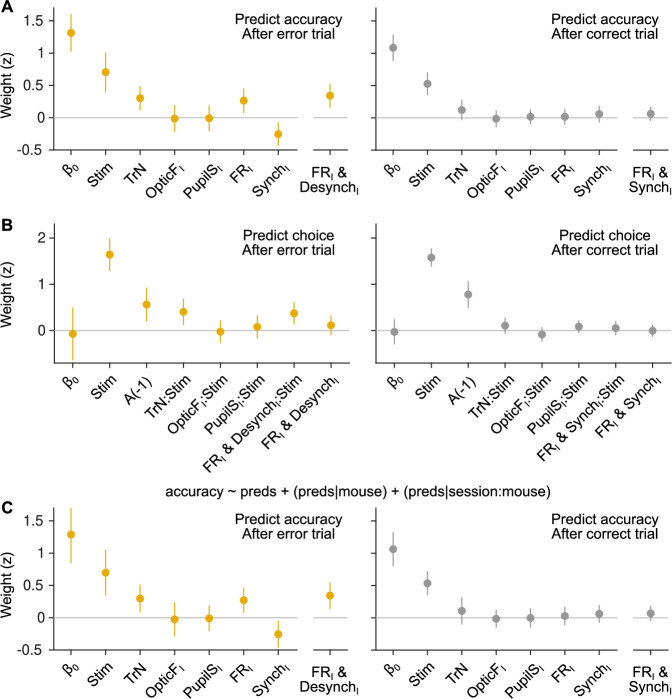
(A) Parametric estimation of confidence intervals (CIs) for accuracy fits. Equivalent to Figure 3C, E, but circle and bars show the mean and 95% CI for each coefficient reported by fitglme (Methods) using an approximation to the conditional mean squared error of prediction (CMSEP) method (Booth and Hobert, 1998). (B) Generalized linear mixed model (GLMM) analysis designed to separately test the effect of cortical state on discriminability (d) and bias (criterion). To do this, we predict the animal’s choice on each trial, not whether the outcome of the trial was correct (as in Figure 3C, E). We used the combined FRI–SynchI predictor which captures, as a single scalar, how favorable the cortical state is for accuracy after errors or correct trials. Considering this predictor as a main effect can capture the effect of cortical state on bias, whereas the interaction between this predictor and the stimulus strength can capture an effect of cortical state on discriminability. Cortical state is only predictive of choice as an interaction term after errors (p = 0.0025). Error bars are computed using parametric estimation. (C) GLMM fit to accuracy computed separately after error trials (left) and correct trials (right) considering recording session as a random effect nested within mouse. Error bars are computed using parametric estimation.
Figure 3—figure supplement 2. Generalized linear mixed model (GLMM) analysis including quadratic terms and differentially for superficial and deep recording shanks.

Figure 3—figure supplement 2.

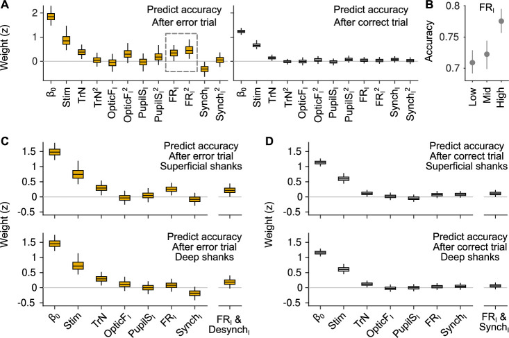
(A) GLMM fit to accuracy for trials following errors (left) and correct responses (right). Differently from the GLMMs in Figure 3, this model includes quadratic terms for TrN, OpticFI, PupilSI, FRI, and SynchI. The only significant quadratic term is the one for FRI after errors. (B) Accuracy as a function of FRI after error trials. The relationship between FRI and accuracy is supralinear and resembles a quadratic function (median and 50% confidence interval [CI] derived using bootstrap), as suggested by the results of the GLMM in (A). (C) GLMM fit to accuracy after error trials using FRI and SynchI predictors that were built using (putative) superficial or deep neurons in the recordings. (D) Same analysis as in (C) but considering only trials after correct responses.
Figure 3—figure supplement 3. Robustness of the results on the effects of cortical state on accuracy.
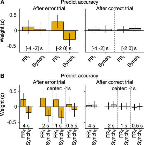
Figure 3—figure supplement 3.

(A) The analysis in Figure 3C–E was repeated but shifting the window 2 s into the past (i.e., window is centered 3 s before stimulus onset, instead of 1 s as in the manuscript). Although the full model was fitted, we only display the magnitude of the firing rate and synchrony innovation predictors. (B) Same but changing the window duration. For the three cases on the right (for each outcome), the center of the window is still at 1 s before the stimulus, as in the manuscript. The first case shows the results for a window [−4 0] s. Overall, these results show that if the window is either too short, or if it moves away too much from the presentation of the sound, the predictive power of baseline activity innovations after errors wanes. However, this (expected) degradation is gradual. Innovations of baseline fluctuations are never predictive of accuracy after correct trials, independently of the window used for measuring baseline activity.
Figure 3—figure supplement 4. Lack of association between slow cortical state fluctuations and accuracy.
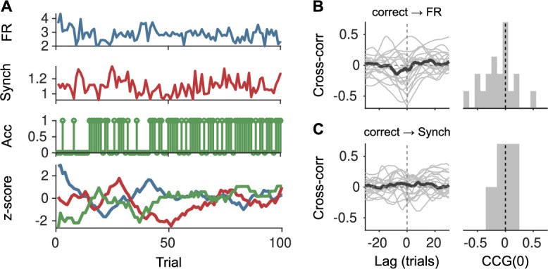
Figure 3—figure supplement 4.

(A) For an example session, we show the raw firing rate (FR; top), Synch (middle top) during the baseline and accuracy (middle bottom) in that trial. Bottom: We smoothed each of these signals with a running window of 10 trials, removed the session-wide linear trend, and z-scored. (B) Left: Cross-correlation function between the smoothed accuracy and FR time series. Each gray line is a recording and the black line is the mean. Right: Histogram across recordings of the cross-correlation function at zero lag. (C) Same as (B) but for the cross-correlation between the smoothed accuracy and Synch time series.
Figure 3—figure supplement 5. Behavioral predictions including slow trends.

Figure 3—figure supplement 5.

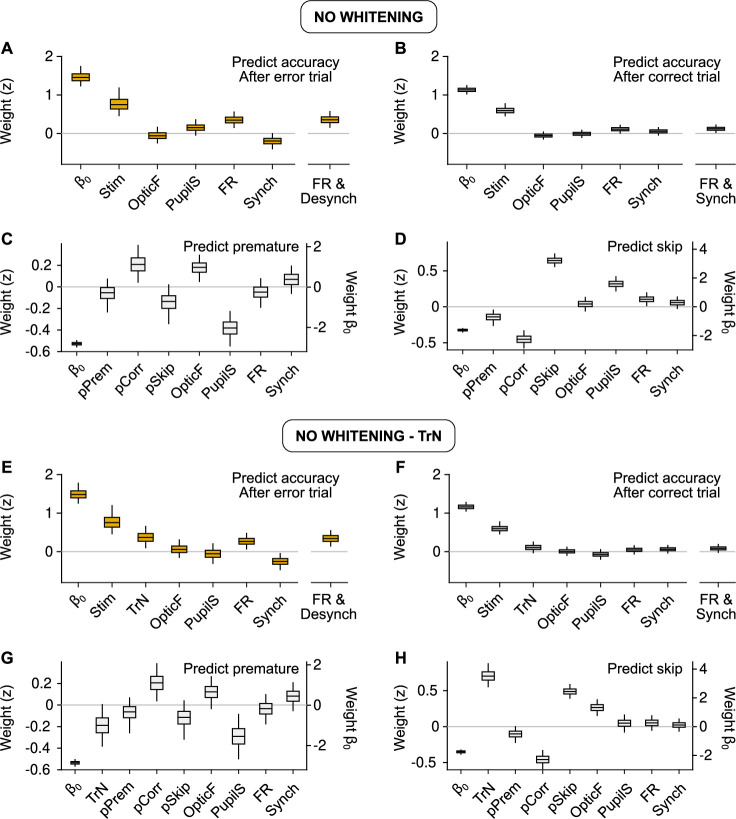
(A, E) Equivalent to Figure 3C (predicting accuracy after errors) but using raw predictors without (A) or with (E) the session trend TrN. (B, F) Same, but equivalent to Figure 3E (predicting accuracy after correct trials). (C, G) Same, but equivalent to Figure 5D (predicting premature trials). (D, H) Same, but equivalent to Figure 5F (predicting Skips). These results are largely equivalent to the ones in the main text using innovations, suggesting that, on average across recordings, slow trends in the baseline signals are not associated in a reliable fashion to accuracy, or the probabilities of premature responding or Skips. If the session trend regressor TrN is not included, the fit to Skips changes, revealing a spurious relationship between Pupil size and Skip probability that arises exclusively by the common increase in both of these variables throughout the session.
Figure 3—figure supplement 6. Outcome dependence of the effect of cortical state on stimulus and choice discriminability from evoked responses.
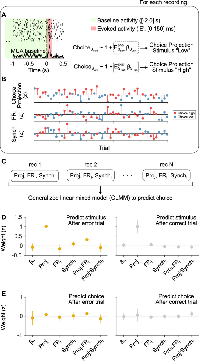
Figure 3—figure supplement 6.

(A) Schematic of our approach. We calculated evoked firing rates in each trial for each neuron in a window of [0 150] ms starting at sound stimulus onset. FRI and SynchI predictors during the [−2 0] s baseline period were the same as in the text. When examining choice discriminability, for each experiment we computed a ‘choice axis’ separately for each of the two stimulus categories using cross-validated regularized logistic regression (see Methods). (B) Using this axis, we computed a scalar ‘choice projection’ for each trial which, together with the baseline regressors FRI and SynchI, constituted the data from each experiment in this analysis. (C) We then aggregated these data from all experiments in a generalized linear mixed model (GLMM) in order to predict choice trial-by-trial, using ‘recording session’ as a random effect. The same exact procedure was used to examine stimulus category discriminability, computing a ‘stimulus axis’ separately for each choice in each recording. (D) Magnitude of the coefficients for each regressor in a GLMM used to predict stimulus category after error (left) and after correct (right) trials. After errors, the interaction between the stimulus projection and FRI is positive and significant (p = 0.002; 95% confidence interval [CI] = [0.12,0.52]) and the median of the interaction between the stimulus projection and SynchI is negative, but not significant (p = 0.40; 95% CI = [−0.32,0.13]). After correct trials, none of the interactions are significant. (E) Same but for choice predictions. Regardless of outcome, the magnitude of the coefficient for the choice projection is not significant, signaling that we cannot detect a non-zero choice probability in our dataset. As expected given the lack of a main effect for the choice projection, the interaction terms with FRI and SynchI are also not significantly different from zero, although the median of the coefficients for each outcome is consistent with the expectation given the results in Figure 3.