CNN-based deep learning method for predicting the disease response to the Neoadjuvant Chemotherapy (NAC) treatment in breast cancer

Abstract

Objective

The objective of the study is to evaluate the performance of CNN-based proposed models for predicting patients' response to NAC treatment and the disease development process in the pathological area. The study aims to determine the main criteria that affect the model's success during training, such as the number of convolutional layers, dataset quality and depended variable.

Method

The study uses pathological data frequently used in the healthcare industry to evaluate the proposed CNN-based models. The researchers analyze the classification performances of the models and evaluate their success during training.

Results

The study shows that using deep learning methods, particularly CNN models, can offer strong feature representation and lead to accurate predictions of patients' response to NAC treatment and the disease development process in the pathological area. A model that predicts ‘miller coefficient’, ‘tumor lymph node value’, ‘complete response in both tumor and axilla’ values with high accuracy, which is considered to be effective in achieving complete response to treatment, has been created. Estimation performance metrics have been obtained as 87%, 77% and 91%, respectively.

Conclusion

The study concludes that interpreting pathological test results with deep learning methods is an effective way of determining the correct diagnosis and treatment method, as well as the prognosis follow-up of the patient. It provides clinicians with a solution to a large extent, particularly in the case of large, heterogeneous datasets that can be challenging to manage with traditional methods. The study suggests that using machine learning and deep learning methods can significantly improve the performance of interpreting and managing healthcare data.

1. Introduction

Research on the applicability of deep learning methods has gained popularity in recent years with the increase in machine performances and the presentation of different alternative methods. Frameworks are tools or libraries that enable faster discovery of presented deep learning models. A convolutional neural network model (CNN) model can take weeks to build a model in the most primitive way when no library or framework is used [[1], [2], [3]]. For this reason, a more efficient model can be created with a tool that includes previously revealed models and optimized parameters [4,5]. Thus, a module open to readability and change is revealed with simplified operations and layer structure [[6], [7], [8], [9], [10]].

Keras library has been chosen for the study [11,12]. Keras, a Python-based deep learning library, is an open-source library and is often preferred in academic research [13]. TensorFlow works as a layer over Microsoft Cognitive Toolkit and Theano libraries [14,15]. It offers an entirely user-friendly approach and enables an expandable structure. With the Tensorflow 2.0 library offered by Google in 2017, Keras has been integrated and brought into a working state [16,17]. Techniques such as data preprocessing and data augmentation can be the reason for preference in obtaining effective results against small datasets. For models such as Inception, MobileNet, and VGG, which are considered to be effective models, pre-trained model weights can be used automatically and easily integrated, thus allowing complex model structures to be established [[18], [19], [20]]. The study includes the evaluation of Neoadjuvant Chemotherapy (NAC), which is applied as a treatment method in patients diagnosed with breast cancer, by using pathological data to estimate the response. In collecting patient data, data related to the relevant case have been obtained from the general surgery and radiology departments of Sakarya Research Hospital through periodic face-to-face interviews with four staff physicians. The data used in the study have been evaluated by obtaining the pathological results of 341 patients in at least one year. Ethics committee approval has been obtained for the use of data, which specialist doctors have supported during the collection and interpretation of data, and the hospital ethics committee also supports the study. In this study, unlike other studies, it is aimed to predict the complete response to treatment using a deep learning model. It has been observed that the number of data is higher than similar studies, which provides an advantage in getting a more accurate estimation.

Nisar et al. in their review article, detailed deep learning models applied to health services to diagnose diseases of the human body system and compared different diseases based on factors and parameters. Different deep learning applications have been compared, and research opportunities and challenges in the related field have been determined. Research on deep learning models in healthcare is extensive, yet many challenges are posed. The questionnaire in the research is aimed to be a step towards the proposed techniques applied in the field of health and these innovations and to lead them to become smarter [21].

Pitale et al. Artificial intelligence (AI) and Deep learning (DL) have become superior problem-solving strategies in many research and industrial applications. Research has explored applications and research areas of deep learning through computer vision in biomedicine and the latest trends in health, safety, education, and technologies [22].

Moghadas et al. although neoadjuvant chemotherapy has been shown as an essential treatment method for locally advanced breast cancer, according to studies, approximately 70% of them can respond positively to treatment. The study investigated machine learning techniques and quantitative computed tomography parametric imaging for early prediction of complete response in treatment. They presented the correlation of tomography images and secondary derivative textural features as a method for estimating before treatment initiation [23].

Byra et al. proposed a learning-based approach in two in-depth studies for early predicting response to neoadjuvant chemotherapy in breast cancer. They showed that in the model presented with pre-trained convolutional neural networks and transfer-learning approaches, response to chemotherapy could be predicted based on ultrasound images collected before treatment. The model is open to development with a larger patient group and data [19].

Both mammography and ultrasound imaging techniques have limited sensitivity and specificity, with limitations in describing lesions that can be partially resolved, especially in the presence of dense breasts. Due to the limitations of all these imaging tools, patients often have to undergo painful and costly biopsy procedures to make a definitive diagnosis. Medical imaging modalities that are invisible to the naked eye and, therefore, significantly emphasize image features increase the discriminatory and predictive potential of medical imaging. However, a 100% accuracy result cannot be achieved in medical images. In this study, the pathological data of patients who have a complete pathological response after NAC (Neoadjuvant Chemotherapy) and can not get the desired result have been used as the data set for the proposed deep learning method. The model has been created with the CNN (Convolutional Neural Network) algorithm, one of the deep learning models, and the predictive performance of the model with new patient data to be submitted to the system has been demonstrated. It has been aimed at developing the model with new data.

2. Materials and method

2.1. Data collection and exploratory data analysis

All methods has been carried out in accordance with relevant guidelines and regulations and all experimental protocols has been approved by Sakarya University Research Hospital. Informed consent has been obtained during the data collection phase [33].

In the research, standardization of the data has been carried out with a preprocessing step before the distribution of pathological data on the data and input to the model. Python programming language was used for modeling and data analysis and Sklearn library was used for data analysis. The variables used for estimating complete pathological response are shown in Table 1. The statistical analysis of the data is shown in Tables 2 and 3.

Table 1.

Dataset variables and annotations.

Variables	Descriptions
millerCoef	Miller coefficient
lnReg	Tumor lymph node value
compltResp	Complete response in both tumor and axilla.
millerPayne	It consists of values between 1 and 5 and a value of 5 indicates that the mass has disappeared, and 1–4 Indicates that it has not disappeared.
age	Age value. It is divided into 3 categorical groups as between 50 and 70.
preopmetsexist	Presence of preoperative metastases.
neosizeUSG	Tumor size before neoadjuvant.
preNeoTumorDiameter	Tumor diameter before neoadjuvant.
preNeoAxilla	Axilla involvement before neoadjuvant.
clinicenfcoef	Clinical infection coefficient
patLN	Presence of axillary lymph node metastases before chemotherapy.
multifoksl	Multifocal-centric, coefficient if more than one in different quadrants.
axilla	Value related to underarm operations
slnsuccess	Slnb, whether a successful sampling can be made, lymph node high low perception and effect value
metsize	Lymph node metastasis size, mini macro moderate categorical values
patmetcoef	Pathological metastasis lymph node coefficient, presence of postoperative lymph node metastasis
metcoef2	Metastasis lymph node coefficient
postneopathsize	Pathology dimension after neoadjuvant
tumorsize	Tumor size after neoadjuvant
grade	Tumor level
clncStgCoef	Clinical stage coefficient
ptnm	Pathological classification
pStgCoef	Pathological stage coefficient
estcoef	Presence of staining
progcoef	Prog coefficient
luminalsubtype	Luminal subtype
ki67coef	Ki 67 coefficient
lenfnod	Extracapsular invasion Tumor invasion beyond the lymph node
lenfinvz	Presence of lymphatic invasion
dvitcoef	Vitamin D coefficient

Table 2.

Statistical distribution of data set variables.

	count	mean	std	min	25%	50%	75%	max
millerCoef	341.0	1.272.727	0.446016	1.0	1.0	1.0	2.0	2.0
lnReg	341.0	0.372434	0.484164	0.0	0.0	0.0	1.0	1.0
compltResp	341.0	0.219941	0.414815	0.0	0.0	0.0	0.0	1.0
millerPayne	341.0	3.234.604	1.417.570	1.0	2.0	3.0	5.0	5.0
age	341.0	1.533.724	0.615635	1.0	1.0	1.0	2.0	3.0
preopmetsexist	341.0	0.099707	0.300049	0.0	0.0	0.0	0.0	1.0
neosizeUSG	341.0	3.700.880	1.580.664	1.0	3.0	3.0	4.0	10.0
preNeoTumorDiameter	341.0	1.920.821	0.560625	1.0	2.0	2.0	2.0	3.0
preNeoAxilla	341.0	0.794721	0.404499	0.0	1.0	1.0	1.0	1.0
clinicenfcoef	341.0	0.821114	0.383820	0.0	1.0	1.0	1.0	1.0
patLN	341.0	0.648094	0.478267	0.0	0.0	1.0	1.0	1.0
multifoksl	341.0	1.416.422	0.700563	1.0	1.0	1.0	2.0	3.0
axilla	341.0	1.747.801	0.844203	1.0	1.0	1.0	3.0	3.0
slnsuccess	341.0	0.692082	0.462311	0.0	0.0	1.0	1.0	1.0
metsize	341.0	2.375.367	0.850524	1.0	2.0	3.0	3.0	3.0
patmetcoef	341.0	0.536657	0.499387	0.0	0.0	1.0	1.0	1.0
metcoef2	341.0	1.671.554	0.769289	1.0	1.0	1.0	2.0	3.0
postneopathsize	341.0	2.140.762	1.508.060	1.0	1.0	2.0	3.0	7.0
tumorsize	341.0	0.580645	0.634851	0.0	0.0	1.0	1.0	2.0
grade	341.0	2.052.786	0.648641	1.0	2.0	2.0	2.0	3.0
clinTNM	341.0	3.378.299	1.481.453	0.0	2.0	3.0	4.0	7.0
clncStgCoef	341.0	2.363.636	0.692203	1.0	2.0	2.0	3.0	4.0
ptnm	341.0	2.413.490	2.054.191	0.0	1.0	2.0	4.0	7.0
pStgCoef	341.0	1.762.463	1.185.401	0.0	1.0	2.0	3.0	4.0
pthgy2	341.0	1.228.739	0.715703	1.0	1.0	1.0	1.0	4.0
estcoef	341.0	0.739003	0.439824	0.0	0.0	1.0	1.0	1.0
progcoef2	341.0	0.630499	0.483379	0.0	0.0	1.0	1.0	1.0
cerb2	341.0	0.319648	0.467025	0.0	0.0	0.0	1.0	1.0
luminalsubtype	341.0	2.085.044	0.914803	1.0	1.0	2.0	3.0	4.0
ki67coef	341.0	2.214.076	0.821355	1.0	1.0	2.0	3.0	3.0
lenfnod	341.0	0.299120	0.458545	0.0	0.0	0.0	1.0	1.0
vasinvas	341.0	0.252199	0.434913	0.0	0.0	0.0	1.0	1.0
lenfinvz	341.0	0.328446	0.470338	0.0	0.0	0.0	1.0	1.0
norinvaz	341.0	0.096774	0.296085	0.0	0.0	0.0	0.0	1.0
dvitcoef	341.0	1.422.287	0.725969	1.0	1.0	1.0	2.0	3.0
dvitcoef2	341.0	1.137.830	0.345228	1.0	1.0	1.0	1.0	2.0

Table 3.

Standardization value labels.

	min	max	Value Labels
millerCoef	1.0	2.0	completeResponse = True: 1; completeResponse = False: 0
age	1.0	3.0	age <50: 1; age <70: 2; age >70: 3
neosizeUSG	1.0	10.0	neosizeUSG ≤ 10:1; neosizeUSG<20:2; …; neosizeUSG>90:10
preNeoTumorDiameter	1.0	3.0	0–2 cm: 1; 2–5 cm: 2; >5 : 3
multifoksl	1.0	3.0	single: 1; multifocal: 2; multicentric: 3
metsize	1.0	3.0	metsize <50: 1; metsize <70: 2; metsize >70: 3
metcoef2	1.0	3.0	1-3: 1; 4–7: 2; >7:3
clinTNM	1.0	7.0	clinicalStage1:1; clinicalStage2a:2; clinicalStage2b:3; ..; clinicalStage3c:7
pthgy2	1.0	4.0	infiltratif duktal ca: 1; infiltratif lobuler ca:2; mix: 3; others:4
luminalsubtype	1.0	4.0	ER, PR +, cerb-: 1; ER/PR/CERB2 +-: 2; triple-negative: 3; Her2 (+): 4
ki67coef	1.0	3.0	<15: 1; 15–29: 2; >29: 3
dvitcoef	1.0	3.0	<20: 1; 20–30: 2; >30: 3
dvitcoef2	1.0	2.0	deficiency: 1; normal: 2

The effecting values for the estimation of response to chemotherapy (Neoadjuvant Complete Response) are given in Table 1, and the total number of patients is 348.

In these data obtained in line with the evaluations of specialist physicians, control (decision) variables (compltResp, millerCoef and lnReg) providing control of the effect on complete response has been determined and their distribution in the data is shown in Fig. 2. In Figure [1 (1–3)], the values and distributions of the decision variables in the dataset have been graphically obtained from histogram analysis.

Fig. 2.

Correlation map between variables.

Discovering and measuring the extent to which the variables in the dataset are interdependent is an essential step in the pre-model process, and this information could help to better prepare the data to meet the expectations of machine learning algorithms such as linear regression, whose performance will decrease with the presence of interdependencies. In Fig. 1., correlations between variables in Fig. 1(1)., 1 (2) and 1 (3). are shown with values ranging from −1 to 1. The correlation between the variables is expressed with a value close to 1 if it is the highest and close to −1 if it is less. The Pearson correlation coefficient calculates the effect on the other variable when one variable changes. This linear relationship can be positive or negative, revealing the relationship between variables, returning values between −1 and 1. It is possible to decide according to this range to measure the strength of two variables. According to the graph, millerPayne, lnReg and millerCoef variables seem to be the variables that most positively coherence to the complete response. On the other hand, it can be discovered from the correlation map as the variables show a negative coherence for metsize, patmetcoef, metcoef2, postneopathsize, ptnm, pStgCoef.

Fig. 1.

Statistical distribution of variables in Panel 1, Panel 2 and Panel 3 in the dataset.

For the complete estimation, the decision variables expected to be estimated according to the results of the field experience and correlation matrix with specialist medical doctors have been created with three different scenarios. While creating the scenarios, the decision variables and neglected variables and scenarios have been determined as Table 4.

Table 4.

Statistical distribution of millerCoef, compltResp and lnReg variables in the dataset.

	Scenario 1	Scenario 2	Scenario 3
Decision variable	compltResp	lnReg	millerCoef
Included variable	–	millerCoef	lnReg
Neglected variable	millerCoef, lnReg	compltResp	compltResp

The variables in Table 4., have been included as input variables, and the compltResp, lnReg and millerCoef variables in the data set have been determined manually by the specialist doctor as decision variables in estimating the course of the disease.

2.2. Proposed deep learning model implemantation

The presence of multiple layers is shown as the main reason for using the expression depth. In traditional machine learning, the number of layers consists of one or two layers and less information is acquired, it is possible to use much more layers in deep learning. The loss function scores the difference between the output from the model and the expected output for each iteration of the model, and the loss function is used as a feedback signal in the next iteration as shown in the flowchart. The weights in the input function are updated again to minimize the loss function. Since a neural network does not have a loss function in its initial position, it is initialized with random initial weight values, Fig. 3. In this case, the loss score will be high since the model's output will be very different from the expected. According to model the model, optimal weight values are where the loss function is minimum and the model prediction rate is the highest. When the optimal values are reached, the loop is terminated, and the lowest loss function is obtained after this flow, called the learning loop.

Fig. 3.

Loss value and weight update in deep learning model.

Input signals in an artificial neural network node are converted as output signals; at this point, the linear function is converted to a nonlinear function, increasing the learning efficiency of the model. As indicated in Fig. 4., the bias value added to the linear function is transmitted to the activation function without obtaining the output value [24].

Fig. 4.

Bias value and activation function.

Model data is divided into 70% training and 30% test set. Suppose the “Scikit” library is not specified with the “train_test_split” function and the random_state parameter called “random_state.” In that case, a new random value is generated each time it is run or executed, and the training and test datasets can have different values each time. In order to prevent this, when another integer constant value such as random_state = 0 or 1 is assigned, the result is the same regardless of how many times the code block is run, so that the same values can be reached in the training and test datasets. The random state parameter ensured that the generated splits were reproducible [25]. Scikit-learn uses random permutations to generate the splits. This ensures that random numbers are generated in the same order.

The model summary in Fig. 5, Fig. 6 is presented according to the estimation process in 2 different classes in all scenarios according to the scenarios in the next section, with 36 variables in Table 1 as input and decision variables. In the model, apart from the input layer and the output layer, it consists of 6 hidden layers, and each layer consists of 128 nodes. The “Relu” activation function is chosen as the activation function among hidden layers, and the “Softmax” activation function is selected in the output layer [25].

Fig. 5.

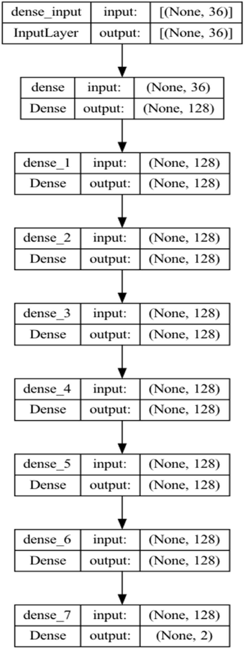
The proposed Keras convulutional model structure.

Fig. 6.

The proposed Keras convulutional model with layer structure.

The Softmax function calculates the probability distribution of the event over ‘n' different events. Generally, this function calculates the probabilities of each target class over all possible target classes; then, the calculated probabilities help determine the target class for the given inputs. The Softmax activation function is the generalized form of the sigmoid function for multiple dimensions and is expressed as in Equation (1) [26].

$$\sigma {\left(\overrightarrow{z}\right)}_i=\frac{e^{z_i}}{\sum _{j=1}^K{e}^{zj}}$$ 1

• $\overrightarrow{z}$: Softmax function input vector consisting of (z0, … zK)

• $z_i$: All zi values are elements of the input vector to the softmax function and can take any real value, positive, zero, or negative.

• $e^{zj}$: The standard exponential function is applied to each element of the input vector, giving a positive value above zero, which is very small if the input is negative and very large if the input is large.

• $K$: Number of classes

ReLU is one of the activation functions used between hidden layers in the model and colud be used in almost all convolutional neural networks or deep learning methods. The Rectified linear activation function, or ReLU for short, is a piecewise linear function that will directly output the input if it is positive. Otherwise, it gives a zero and is shown in Equations 2, 3) [27].

$$g\left(x\right)=\{\begin{array}{cc}x& x>0\\ 0& x<0\end{array}$$ 2

$$g^{\prime }\left(x\right)=\{\begin{array}{cc}1& x>0\\ 0& x<0\end{array}$$ 3

In the model, the “epoch” number is 240 and the “batch_size” number is 16, and the results are evaluated by observing in all three scenarios. The “epoch” number refers to the completion of an artificial neural network's forward propagation and backpropagation process. “Batch_size” refers to the number of training samples in the forward propagation or backpropagation process; an increase in this number also increases the memory usage resource and can lead to performance results in model training. On the other hand, the number of iterations is evaluated by evaluating the forward propagation and backpropagation processes separately, regardless of the batch number. Assuming 1000 samples as training data and considering the batch size as 500, two iterations are needed to complete one epoch.

When the training model is run more than the optimal level, it may minimize total cost and result in overfitting. In this case, while the classification success rate obtained in the training set is high, lower values can be obtained in the test set. It is obtained with a high variance and a low bias value. In order to prevent this situation, it may be advantageous to reduce the number of high features and to delete the highly correlated variables or to create a model with a single new variable. It is possible to avoid this situation with a high level of data. In the opposite case, it is considered the main goal for the model to learn from the training data, but it is desired to be trained less, so it may be a solution to stop the training process earlier. However, if the model needs to learn more from the training data, it may not even catch the dominant trend.

3. Results

Scenario 1 (compltResp estimation) variables and model result accuracy value and loss value are obtained as in the graphs below. The graphs with the number of epochs in the model and the training and validation values obtained at each step are given in Fig. 7, Fig. 8.

Fig. 7.

Scenario 1 epoch accuracy graph.

Fig. 8.

Scenario 1 Loss chart.

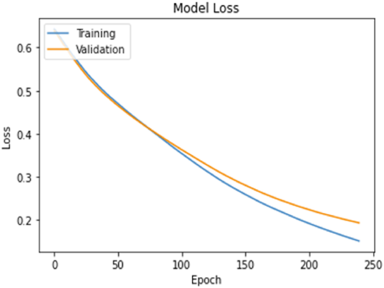
The model accuracy and loss graphs with the number of epochs in the scenario 2 (lnReg estimation) model and the training and validation values obtained at each step are given in Fig. 9, Fig. 10.

Fig. 9.

Scenario 2 epoch accuracy graph.

Fig. 10.

Scenario 2 Loss chart.

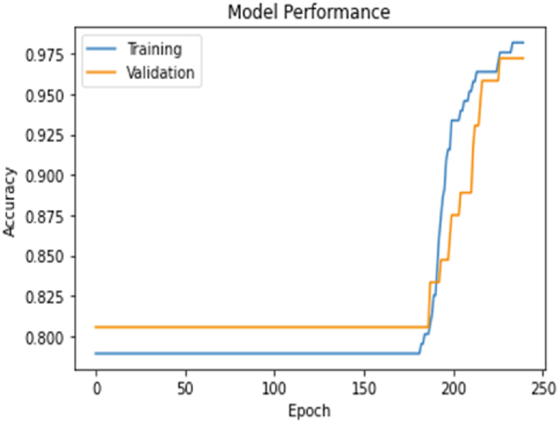
The number of epochs with the scenario 3 (millerCoef) model and the training and verification values obtained in each step and the model accuracy and loss graphs are given in Fig. 11, Fig. 12.

Fig. 13.

Scenario test data classification distribution.

Fig. 11.

Scenario 3 epoch accuracy graph.

Fig. 12.

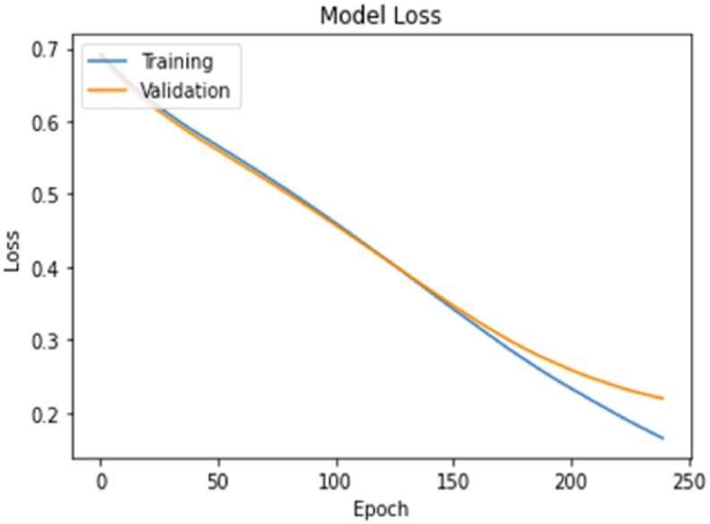
Scenario 3 Loss chart.

Considering the estimation accuracy and loss values in the scenarios according to the model, the decision variable estimation success in scenario 3 has the highest with 91% success.

Because the unbalanced distribution of the decision variables in the data and the TN (True Negative) ratio in the estimation should be considered as a more critical evaluation criterion. For this reason, the confusion matrix and evaluation metrics for each scenario have been obtained as in Figure [13 (1–3)] and Table 5. When the metrics are evaluated, it is seen that the highest performance of the TN ratio estimation was obtained with a score of 84% in the estimation of the millerkat variable, which is the estimation variable in Scenario 3 as shown in Figure [13 (3)].

Table 5.

Scenarios classification performance summary metrics.

	Precision	Recall	F1 Score
Scenario 1	1.0	0.77	0.87
Scenario 2	1.0	0.68	0.77
Scenario 3	1.0	0.84	0.91

AUC — ROC rotation provides an extra performance measure for the difficulty problem at various threshold settings [28]. ROC is an expansion and represents the grade or size of AUC races [29]. AUC is the area under the ROC bend (source) as shown Figure [14 (1–3)]. We find that the higher the AUC, the better the model predicts, and the area under the curve in scenario three is also seen in Fig. 14(3), where it is the largest.

Fig. 14.

AUC — ROC metrics.

The ROC curve is frequently used in the literature to compare models. However, the most commonly used are accuracy, recall, precision, and F1 score. There is a class imbalance in the variables in the three scenarios determined as the evaluation criteria in the study. For this reason, accuracy and F1 scores are sensitive in unbalanced data. As a different approach in binary classification, Matthews Correlation Coefficient (MCC) method offers a more realistic measurement metric in asymmetric data (source) [[30], [31], [32]]. In Fig. 15, MCC values have been obtained as 84%, 65%, and 88%, respectively, in the scenarios.

Fig. 15.

Matthews Correlation Coefficient (MCC) and negative forecast performance evaluation.

4. Conclusion

In this study, a deep learning model has been proposed to predict pathological complete response after neoadjuvant chemotherapy treatment. A user-friendly interface application can enable physicians to identify high-risk patients who need a specific therapeutic scheme with easier prediction and evaluation of treatment response for patients after NAC therapy. However, further data and validation studies are required to further develop this model and clinical treatment.

Healthcare institutions produce big heterogeneous data in different structures and sources daily. Depending on the situation, the prediction of being able to make sense of and manage the data in this structure with traditional methods may decrease. It is a powerful tool for managing, interpreting, and analyzing such data with machine learning and deep learning methods. In a clinical practice called prognosis, estimating a disease's development process includes making predictions such as worsening, improving, or stabilizing the course of the disease according to the conditions.

It is a powerful tool for managing, interpreting, and analyzing such data with machine learning and deep learning methods. In a clinical practice called prognosis, estimating a disease's development process includes making predictions such as worsening, improving, or stabilizing the course of the disease according to the conditions.

In determining the correct diagnosis and treatment method with the prognosis follow-up of the patient, different types of data such as pathological test results, radiological images, and interpretation of the data stored in different sources with deep learning methods provide clinicians with a solution to a large extent. Fully automatic intelligent medical image diagnostic systems are expected to be a part of the following generation of health systems.

The data used in the study consists of data specifically for a specific patient group processed depending on the permission of the ethics committee. Although a standard information system has been established in order to protect the integrity of the processed data and to ensure data continuity, the storage and standardization of data specific to a specific disease is an area open to development.

Building deep learning models for clinical decision support systems often requires the systematic collection of large amounts of data, which is time-consuming and requires significant human effort. Even though medical data is collected carefully on a case-by-case basis under normal conditions, many factors can disrupt the correct (expected) functionality of the data needed in deep learning systems. Instrumental and environmental noises can affect the collected data, thus increasing the risk of misdiagnosis. In the study, with the pre-processing step of the pathological data, the data in the disorder that could affect the model have been eliminated in the company of the physicians. It turns out that the clinical usability of AI-powered systems depends on the development of data-driven healthcare.

Declarations

Funding

Authors did not receive any funding.

Data availability statement

Provided by the corresponding author on request and can be contacted via mail.

Code availability

Available on request.

Authors' contributions

All authors have contributed equally to the conception and design of the study, the acquisition and analysis of data, and the drafting and critical revision of the manuscript. All authors have provided final approval of the version submitted.

Declaration of competing interest

The authors declare that they have no known competing financial interests or personal relationships that could have appeared to influence the work reported in this paper.

References

- 1.Miotto R., Wang F., Wang S., Jiang X., Dudley J.T. Deep learning for healthcare: review, opportunities and challenges. Briefings Bioinf. 2018;19:1236–1246. doi: 10.1093/bib/bbx044. [DOI] [PMC free article] [PubMed] [Google Scholar]
- 2.Sengupta S., Basak S., Saikia P., Paul S., Tsalavoutis V., Atiah F., Ravi V., Peters A. A review of deep learning with special emphasis on architectures, applications and recent trends. Knowl. Base Syst. 2020;194 doi: 10.1016/j.knosys.2020.105596. [DOI] [Google Scholar]
- 3.Kim K.G. Book review: deep learning. Healthc. Inform. Res. 2016;22:351. doi: 10.4258/hir.2016.22.4.351. [DOI] [Google Scholar]
- 4.Zhu X.X., Tuia D., Mou L., Xia G.-S., Zhang L., Xu F., Fraundorfer F. Deep learning in remote sensing: a comprehensive review and list of resources. IEEE Geosci. Remote Sens. Mag. 2017;5:8–36. doi: 10.1109/MGRS.2017.2762307. [DOI] [Google Scholar]
- 5.Min S., Lee B., Yoon S. Deep learning in bioinformatics. Briefings Bioinf. 2016:bbw068. doi: 10.1093/bib/bbw068. [DOI] [PubMed] [Google Scholar]
- 6.Alzubaidi L., Zhang J., Humaidi A.J., Al-Dujaili A., Duan Y., Al-Shamma O., Santamaría J., Fadhel M.A., Al-Amidie M., Farhan L. Review of deep learning: concepts, CNN architectures, challenges, applications, future directions. J. Big Data. 2021;8:53. doi: 10.1186/s40537-021-00444-8. [DOI] [PMC free article] [PubMed] [Google Scholar]
- 7.Chen H., Chen A., Xu L., Xie H., Qiao H., Lin Q., Cai K. A deep learning CNN architecture applied in smart near-infrared analysis of water pollution for agricultural irrigation resources. Agric. Water Manag. 2020;240 doi: 10.1016/j.agwat.2020.106303. [DOI] [Google Scholar]
- 8.Rusk N. Deep learning. Nat. Methods. 2016;13:35. doi: 10.1038/nmeth.3707. 35. [DOI] [Google Scholar]
- 9.LeCun Y., Bengio Y., Hinton G. Deep learning. Nature. 2015;521:436–444. doi: 10.1038/nature14539. [DOI] [PubMed] [Google Scholar]
- 10.Maruyama T., Hayashi N., Sato Y., Hyuga S., Wakayama Y., Watanabe H., Ogura A., Ogura T. Comparison of medical image classification accuracy among three machine learning methods. J. X Ray Sci. Technol. 2018;26:885–893. doi: 10.3233/XST-18386. [DOI] [PubMed] [Google Scholar]
- 11.Khan A., Sohail A., Zahoora U., Qureshi A.S. A survey of the recent architectures of deep convolutional neural networks. Artif. Intell. Rev. 2019;53:5455–5516. doi: 10.1007/s10462-020-09825-6. [DOI] [Google Scholar]
- 12.Soniya S.Paul, Singh L. 2015 IEEE Work. Comput. Intell. Theor. Appl. Futur. Dir., IEEE. 2015. A review on advances in deep learning, içinde; pp. 1–6. [DOI] [Google Scholar]
- 13.Schmidhuber J. Deep learning in neural networks: an overview. Neural Network. 2015;61:85–117. doi: 10.1016/j.neunet.2014.09.003. [DOI] [PubMed] [Google Scholar]
- 14.Mathew A., Amudha P., Sivakumari S. Deep learning techniques: an overview. içinde. 2021:599–608. doi: 10.1007/978-981-15-3383-9_54. [DOI] [Google Scholar]
- 15.Angermueller C., Pärnamaa T., Parts L., Stegle O. Deep learning for computational biology. Mol. Syst. Biol. 2016;12:878. doi: 10.15252/msb.20156651. [DOI] [PMC free article] [PubMed] [Google Scholar]
- 16.Niu Z., Zhong G., Yu H. A review on the attention mechanism of deep learning. Neurocomputing. 2021;452:48–62. doi: 10.1016/j.neucom.2021.03.091. [DOI] [Google Scholar]
- 17.Khamparia A., Singh K.M. A systematic review on deep learning architectures and applications. Expet Syst. 2019;36 doi: 10.1111/exsy.12400. [DOI] [Google Scholar]
- 18.Cao C., Liu F., Tan H., Song D., Shu W., Li W., Zhou Y., Bo X., Xie Z. Deep learning and its applications in biomedicine, genomics. Proteom. Bioinfor. 2018;16:17–32. doi: 10.1016/j.gpb.2017.07.003. [DOI] [PMC free article] [PubMed] [Google Scholar]
- 19.Byra M., Dobruch-Sobczak K., Klimonda Z., Piotrzkowska-Wroblewska H., Litniewski J. Early prediction of response to neoadjuvant chemotherapy in breast cancer sonography using siamese convolutional neural networks. IEEE J. Biomed. Heal. Informatics. 2021;25:797–805. doi: 10.1109/JBHI.2020.3008040. [DOI] [PubMed] [Google Scholar]
- 20.Ching T., Himmelstein D.S., Beaulieu-Jones B.K., Kalinin A.A., Do B.T., Way G.P., Ferrero E., Agapow P.-M., Zietz M., Hoffman M.M., Xie W., Rosen G.L., Lengerich B.J., Israeli J., Lanchantin J., Woloszynek S., Carpenter A.E., Shrikumar A., Xu J., Cofer E.M., Lavender C.A., Turaga S.C., Alexandari A.M., Lu Z., Harris D.J., DeCaprio D., Qi Y., Kundaje A., Peng Y., Wiley L.K., Segler M.H.S., Boca S.M., Swamidass S.J., Huang A., Gitter A., Greene C.S. Opportunities and obstacles for deep learning in biology and medicine. J. R. Soc. Interface. 2018;15 doi: 10.1098/rsif.2017.0387. [DOI] [PMC free article] [PubMed] [Google Scholar]
- 21.Nisar D.E.M., Amin R., Shah N.U.H., Ghamdi M.A.A., Almotiri S.H., Alruily M. Healthcare techniques through deep learning: issues, challenges and opportunities. IEEE Access. 2021;9 doi: 10.1109/ACCESS.2021.3095312. –98541. [DOI] [Google Scholar]
- 22.Pitale R., Kale H., Kshirsagar S., Rajput H. A schematic review on applications of deep learning and computer vision. Asian Conf. Innov. Technol. ASIANCON. 2021;2021(2021) doi: 10.1109/ASIANCON51346.2021.9544941. [DOI] [Google Scholar]
- 23.Moghadas-Dastjerdi H., Rahman S.E.T.H., Sannachi L., Wright F.C., Gandhi S., Trudeau M.E., Sadeghi-Naini A., Czarnota G.J. Prediction of chemotherapy response in breast cancer patients at pre-treatment using second derivative texture of CT images and machine learning. Transl. Oncol. 2021;14 doi: 10.1016/J.TRANON.2021.101183. [DOI] [PMC free article] [PubMed] [Google Scholar]
- 24.Ding B., Qian H., Zhou J. 2018 Chinese Control Decis. Conf., IEEE. 2018. Activation functions and their characteristics in deep neural networks, içinde; pp. 1836–1841. [DOI] [Google Scholar]
- 25.Aurélien Géron, Hands-On Machine Learning with Scikit-Learn, Keras, and TensorFlow: Concepts ... - Aurélien Géron - Google Kitaplar, y.y. https://books.google.com.tr/books?hl=tr&lr=&id=HnetDwAAQBAJ&oi=fnd&pg=PT9&dq=Hands-On+Machine+Learning+with+Scikit-Learn+and+TensorFlow&ots=kPUxFLxKyb&sig=St-v6r3S614HyHN6PBEW_7SGffg&redir_esc=y#v=onepage&q=Hands-On Machine Learning with Scikit-Learn and TensorFlow&f=false (erişim 20 Mart 2022).
- 26.Softmax Function Definition | DeepAI, (y.y.). https://deepai.org/machine-learning-glossary-and-terms/softmax-layer (erişim 20 Mart 2022).
- 27.Activation Functions in Neural Networks | By SAGAR SHARMA | Towards Data Science, (y.y.). https://towardsdatascience.com/activation-functions-neural-networks-1cbd9f8d91d6 (erişim 20 Mart 2022).
- 28.Lobo J.M., Jiménez-Valverde A., Real R. AUC: a misleading measure of the performance of predictive distribution models. Global Ecol. Biogeogr. 2008;17:145–151. doi: 10.1111/j.1466-8238.2007.00358.x. [DOI] [Google Scholar]
- 29.Huang Jin, Ling C.X. Using AUC and accuracy in evaluating learning algorithms. IEEE Trans. Knowl. Data Eng. 2005;17:299–310. doi: 10.1109/TKDE.2005.50. [DOI] [Google Scholar]
- 30.Awoyemi J.O., Adetunmbi A.O., Oluwadare S.A. Int. Conf. Comput. Netw. Informatics, IEEE. 2017. Credit card fraud detection using machine learning techniques: a comparative analysis, içinde: 2017; pp. 1–9. [DOI] [Google Scholar]
- 31.Jones D.T., Ward J.J. Prediction of disordered regions in proteins from position specific score matrices. Proteins Struct. Funct. Genet. 2003;53:573–578. doi: 10.1002/prot.10528. [DOI] [PubMed] [Google Scholar]
- 32.Saqlain S.M., Sher M., Shah F.A., Khan I., Ashraf M.U., Awais M., Ghani A. Fisher score and Matthews correlation coefficient-based feature subset selection for heart disease diagnosis using support vector machines. Knowl. Inf. Syst. 2019;58:139–167. doi: 10.1007/s10115-018-1185-y. [DOI] [Google Scholar]
- 33.Ethical Clearance Document, GitHub. Available at: https://github.com/kirelli/EthicalClearance/blob/main/EthicalClearance.jpg (Accessed: April 1, 2023)..
Associated Data
This section collects any data citations, data availability statements, or supplementary materials included in this article.