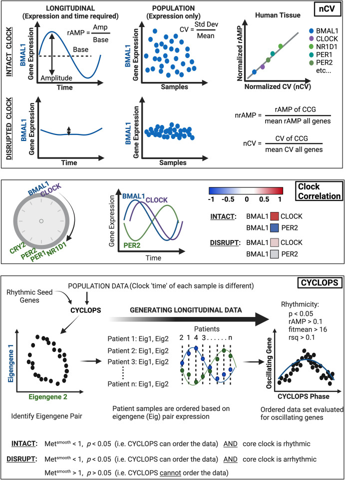
Fig 1. Bioinformatics pipeline for circadian function.
Recently, there have been three separate bioinformatics tools that have substantially improved the ability to determine circadian clock function in population-level transcriptional data [22,25–28]. Normalized coefficient of variation (nCV): Clock gene expression produces robust oscillations with the amplitude of the oscillation defined by the difference between peak and trough, and relative amplitude (rAMP) determined by the ratio between amplitude and baseline level of expression (upper left). Clock disruption (such as with clock gene knockout) causes suppressed rAMP, and thus rAMP can be considered a strong determinant of clock function (lower left). Because rAMP is calculated from time-labeled samples, it can only be measured in human population data when sample time acquisition is known (e.g., MetaCycle) or when using programs to predict longitudinal time-course data (e.g., CYCLOPS). To overcome this limitation and assess core clock gene ‘robustness’ of oscillation in human data (without labeled time), normalized coefficient of variation (nCV) is used. The nCV is the coefficient of variation (CV) of the core clock gene (in the population data) divided by the mean CV of all genes in the dataset. And the CV is determined by the standard deviation of the gene expression divided by its average expression. Thus, when the circadian clock is intact, circadian genes in large population data sets would be expected to have a relatively high nCV due to oscillating gene expression (upper middle). Conversely, with a disrupted clock, the variation of the core clock genes would be diminished (oscillation is suppressed), resulting in a relatively low nCV (lower middle). Importantly, the nCV was found–across multiple cancer types and tissues–to correspond directly to the normalized rAMP (upper right) [25]; it can thus be used confidently as a surrogate for rAMP, which is a key determinant of clock health. Of note, the rAMP (and thus nCV) of core clock genes differs due to differences in amplitude, and so the between tissue difference (e.g., normal vs cancer) for each core clock gene is the value of importance. Clock Correlation: When the circadian clock is intact, there is an expected progression of core clock gene expression, where the positive arm of the clock (e.g., BMAL1, CLOCK) drives transcription of the negative arm of the clock (e.g., PER, CRY). Thus, when BMAL1 expression peaks, CLOCK expression should also be near its peak, and this should be evident in population-level data (i.e., can look at the spread of individual expression points across the population). In turn, when BMAL1 expression peaks, negative arm members (e.g., PER1-2) should be at a trough. Concordantly, strong positive correlations (0.5 < ρ < 1, red) should be apparent among transcriptional activators (e.g., BMAL1 and CLOCK) and among transcriptional repressors (e.g., NR1D1 and PER2), and a strong negative correlation (-0.5 > ρ > -1, blue) should be present amongst activators and repressor targets (e.g., BMAL1 and PER2). If this is the case, then the clock is intact; if these correlations are not preserved (i.e., ρ ~ 0), this indicates the clock is disrupted. Using the set of core clock genes and clock-associated genes, the correlation of each gene against the others is determined by Spearman’s rho (ρ) and mapped in matrix form. This experimental matrix is then compared to a baseline correlation matrix from the mouse circadian gene atlas using the Mantel test, which compares the correlation between the two matrices to produce a z-statistic (z-stat). A higher z-stat value corresponds to a correlation matrix that is closer to the circadian gene atlas baseline (i.e., highly preserved clock correlation). CYCLOPS: Intrinsic to circadian clock genes is rhythmic expression. CYCLOPS (cyclic ordering by periodic structure) is an algorithm that can identify rhythmic (longitudinal) data from population data where sample time acquisition is unknown. The basis for this type of program is that each sample has a different ‘clock time’ due to differences in time of sample acquisition and environmental factors such as sleep/wake cycle or shift worker status (e.g., 15–20% of patients are night shift workers). Seed genes that are known to be rhythmic in the tissue of interest (i.e., pancreas) are inputted into CYCLOPS, and the population level data is reduced to two vectors (Eigengene 1 and Eigengene 2) derived from the seed genes. When plotted, the optimal Eigengene pair will demonstrate an ellipse, which indicates that the two Eigengenes are rhythmic and anti-phasic–this pair can then be used for each patient sample to determine the sample ‘time’, and thus the order of that sample relative to the 24-hr period (phase). By incorporating enough patients, population-level data can be transformed into longitudinal data. Subsequently, with the patient sample dataset ordered by CYCLOPS (by the Eigengene pair), individual genes (e.g., oscillating genes or core clock genes) can be evaluated for rhythmicity. An intact circadian clock is indicated by the ability of CYCLOPS to order the data (statistically) and the identification of rhythmically expressed core clock genes. Meanwhile, a disrupted clock is designated as arrhythmic core clock gene expression or an inability of CYCLOPS to order the data (statistically). Statistically significant rhythmic gene expression is determined by p < 0.05, rAMP > 0.1, fitmean > 16 and goodness of fit (rsq) > 0.1. The fitmean value can be conceptualized as a mean level of expression of that gene across the dataset, and therefore a minimum level of expression (fitmean > 16) is required for rhythmicity cutoff. The goodness of fit of the experimental values by cosinor regression is calculated by R squared (rsq). CYCLOPS reordering is assessed by the Metsmooth and Staterr (significant reordering: Metsmooth < 1 and Staterr < 0.05). The Metsmooth compares the smoothness of the reconstructed circular trajectory versus a linear ordering based on the first principal component, while the Staterr (we designate as p-value) is analogous to the F statistic of a typical nested regression and compares the model fit when a circular rather than linear bottleneck node is used. A full mathematical derivation has been previously outlined by Anafi et al. [28] Figure created with BioRender.com.

