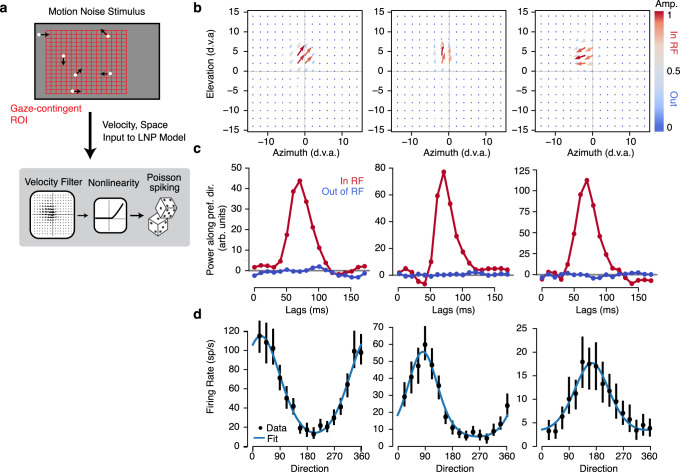
Fig. 3. Receptive field mapping and tuning in MT.

a Sparse motion-noise stimulus was converted into a spatiotemporal velocity stimulus with separate horizontal and vertical velocities using a gaze-contingent grid with 2° spacing. This downsampled stimulus is used to estimate the receptive field (RF) using linear nonlinear Poisson model (LNP). b The spatial map at the peak lag of the spatiotemporal velocity RF from the LNP fits is shown as a vector plot for three example units. Color indicates the vector amplitude (ranging from 0 to 1, with gray at 0.5). c The temporal impulse response was measured both in and out of the RF by projecting the (unnormalized) vector at the maximum and minimum amplitude of the spatial RF on the preferred direction (unit vector). The three plots correspond to the three example units in b. d Tuning curves were measured by masking the stimulus with half of the max of the spatial RF and computing the mean firing rate at the peak lag for each direction shown. Error bars are 95% confidence intervals measured with bootstrapping and blue lines are fits with a von mises function.