Figure 4.

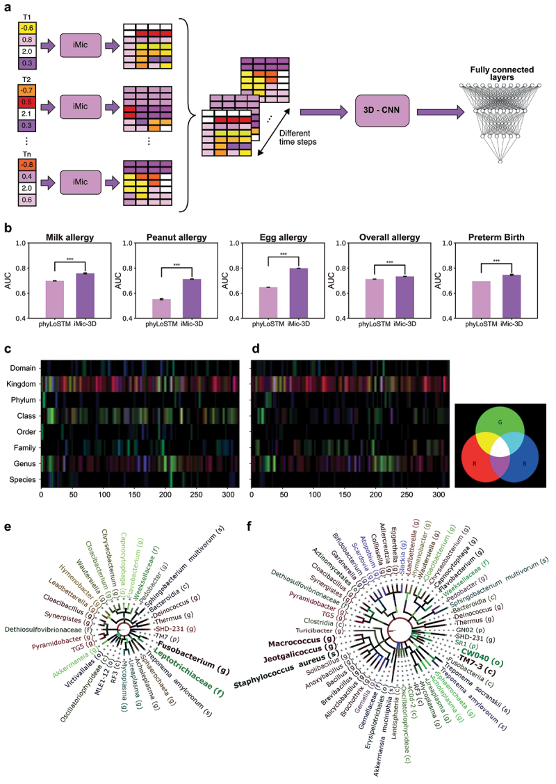
3D learning.

(a) iMic 3D Architecture: The ASV frequencies of each snapshot are preprocessed and combined into images as in the static iMic. The images from the different time points are combined into a 3D image, which is the input of a 3-dimensional CNN followed by two fully connected layers that return the predicted phenotype. (b) Performance of 3D learning vs PhyLoSTM. The AUCs of the 3D-iMic are consistently higher than the AUCs of the phyLoSTM on all the tags and datasets we checked $(n=5)$. The standard errors among the CVs are also shown. phyLoSTM is the current state-of-the-art for these datasets (two-sided T-test, $p$-value $<0.0005$). To visualize the three-dimensional gradients (as in Figure 3), we studied a CNN with a time window of 3 (i.e., 3 consecutive images combined using convolution). We projected the Grad-Cam images to the R, G, and B channels of an image. Each channel represents another time point where R = earliest, G = middle, and B = latest time point. (c,d) Images after Grad-Cam: Each pixel represents the value of the backpropagated gradients after the CNN layer. The 2-dimensional image is the combination of the three channels above. (i.e., the gradients of the first/second/third time step are in red/green/blue). The left image is for normal birth subjects in the DiGiulio dataset, and the right image is for pre-term birth subjects. (e,f) Grad-Cam projection. Projection of the above heatmaps on the cladogram as in Figure 3. The taxa in bold are important taxa that are consistent with the literature.