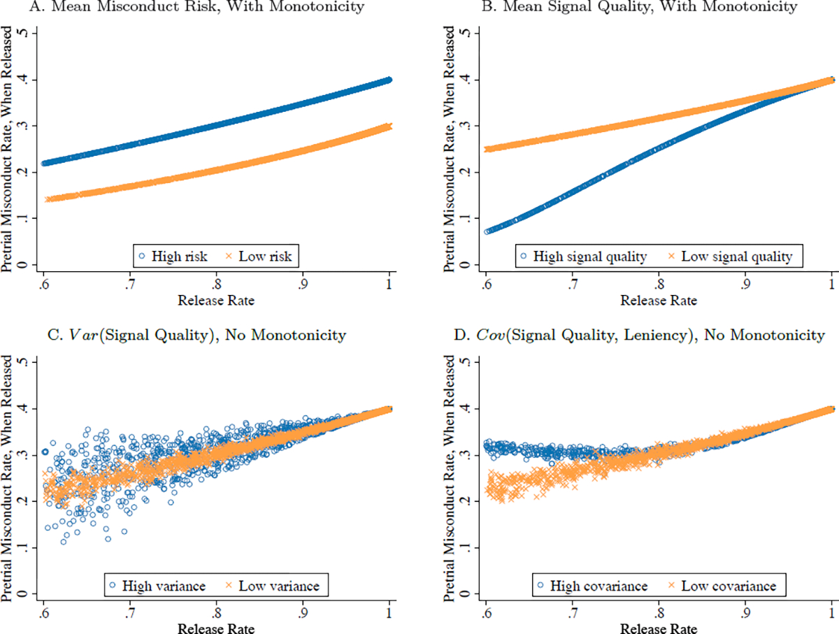
Figure 5:

Identification of Hierarchical MTE Model Parameters

Notes. This figure plots simulated race- and judge-specific release rates against rates of pretrial misconduct among the set of released defendants under different parameterizations of the hierarchical MTE model described in the text. Panel A plots differences in mean misconduct risk (μ = 0.4 vs. μ = 0.3) when conventional MTE monotonicity holds (ψ = 0). Panel B plots differences in mean signal quality (α = 1 vs. α = 0) when conventional MTE monotonicity holds (ψ = 0). Panel C plots differences in signal quality variance (ψ = 0.4 vs. ψ = 0.1). Panel D plots differences in the covariance between judge signal quality and judge leniency (β = 2 vs. β = 0.1). The default parameterization is μ = 0.4, α = 0.2, ψ = 0.1, β = 0, γ = 1.3, and δ = 1.