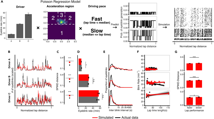
Figure 3.
Three regressors in a Poisson generalized linear model (GLM) replicate many features of eyeblinks during Formula car driving
(A) A Poisson GLM model with three regressors: individuals, acceleration region, and lap driving pace predict the moment-by-moment probability of eyeblinks (one lap is represented by one thin gray line) (middle right). We simulated data by generating random values corresponding to each telemetry data moment that followed a binomial distribution with p = (predicted moment-by-moment probability) and n = 1. A raster plot for one simulated dataset is shown on the right.
(B–G) Signatures of one simulated eyeblink dataset (red) and real data (black). Similar to Figure 1, but for (B), a spatial histogram of eyeblink count is used instead of a raster plot. (C) SPIKE-distance of actual data (black circle), surrogate data generated from actual data (gray violin plot), and mean SPIKE-distance of 20 simulated datasets (red circle). Asterisks indicate the nonparametric statistical significance of the synchronization level of the simulated mean SPIKE-distance compared to the actual surrogate data. (D) Eyeblink rates of actual and simulated data. The error bar indicates one standard error. (E) Actual and simulated histograms of interblink-interval frequency. (F) Correlation between lap time length and blink rate in each lap for actual and simulated data. (G) Piecewise SPIKE-distances within faster and slower laps. Error bars indicating across-lap mean SEM. Asterisks indicate statistically significant differences between conditions using the notation: n.s. for not significant, ∗ for p < 0.05 and ∗∗∗ for p < 0.001.

