MULTIMODAL MICROSCOPY IMAGE ALIGNMENT USING SPATIAL AND SHAPE INFORMATION AND A BRANCH-AND-BOUND ALGORITHM

Abstract

Multimodal microscopy experiments that image the same population of cells under different experimental conditions have become a widely used approach in systems and molecular neuroscience. The main obstacle is to align the different imaging modalities to obtain complementary information about the observed cell population (e.g., gene expression and calcium signal). Traditional image registration methods perform poorly when only a small subset of cells are present in both images, as is common in multimodal experiments. We cast multimodal microscopy alignment as a cell subset matching problem. To solve this non-convex problem, we introduce an efficient and globally optimal branch-and-bound algorithm to find subsets of point clouds that are in rotational alignment with each other. In addition, we use complementary information about cell shape and location to compute the matching likelihood of cell pairs in two imaging modalities to further prune the optimization search tree. Finally, we use the maximal set of cells in rigid rotational alignment to seed image deformation fields to obtain a final registration result. Our framework performs better than the state-of-the-art histology alignment approaches regarding matching quality and is faster than manual alignment, providing a viable solution to improve the throughput of multimodal microscopy experiments.

1. INTRODUCTION

Integrating multiple modes of experimental technologies, such as neuronal functional activity and gene expression from the same population of neurons, can significantly enhance our understanding of cell types in the brain [1, 2, 3, 4, 5, 6, 7]. However, despite the increased availability of such data, techniques that map between multimodal images are lacking. The main challenge is that the source and target images have significantly different appearances, due to, e.g., tissue shrinkage and expansion, signal loss, and other distortions which occur during the experimental process. Furthermore, in many datasets, different subsets of cells may be labeled in each modality, which complicates the matching and alignment process.

A relevant but simpler problem is histology image registration with differently-stained tissues. A recent challenge [8] concluded that even for this easier problem, off-the-shelf registration techniques fail to capture the correct alignment. Specialized approaches for histology images alignment have been developed since then [9], but they are not applicable to multimodal imaging which uses different microscopes and chemical reagents. As a result, many of the recent multimodal studies have used additional landmarks [10] (fiducial markers) and are highly dependent on manual alignment, which is time-consuming, error-prone, and lacks objectivity [5, 2, 11, 6, 7].

In this paper, we present a novel computational framework that automatically aligns a population of neurons from multimodal images taken from mouse brains, without the necessity of fiducial markers or manual pre-alignment. Our main technical contribution is that we cast the multimodal neural alignment problem as a point-cloud subset matching problem and provide an efficient branch-and-bound algorithm to find a globally optimal solution. Furthermore, to prune the combinatorial branch-and-bound search tree, we find locally matching cells using complementary information about cell shapes and locations. Finally, given the presence of non-rigid deformations in the images that typically arise in experimental conditions, we further refine our solution using a pass of deformable registration.

Our algorithmic approach and the heuristics that improve its efficiency provide a viable solution to the multimodal microscopy alignment problem, which had not been addressed in previous work, with novel applications in neuroscience. We demonstrate the performance of our approach in both simulated and real multimodal microscopy imaging experiments captured from the mouse hippocampus [2]. Furthermore, we show that our approach is more accurate than leading histology alignment techniques [8, 12, 13] and is less time-consuming than manual registration. The code, details of the algorithm, and datasets are available at https://github.com/ShuonanChen/multimodal_image_registration.git

2. METHODS

Notation:

First, we introduce the notation used in the paper. Let $S\in {\mathbb{R}}^{d_1^S\times d_2^S\times d_3^S}$ and $T\in {\mathbb{R}}^{d_1^T\times d_2^T\times d_3^T}$ denote the source and target 3D image volumes, and let $\hat{S}\in {\mathbb{R}}^{d_1^T\times d_2^T\times d_3^T}$ denote the transformed source image that matches with the target image. Let $s\in \{1,\dots M{\}}^{d_1^S\times d_2^S\times d_3^S}$ and $t\in \{1,\dots N\}{\}}^T\times d_2^T\times d_3^T$ denote the segmentation maps of $S$ and $T$, that capture $M$ and $N$ cells in the source and target volumes, respectively. Local patches surrounding each cell are denoted as ${\mathbf{Q}}_i^s,{\mathbf{Q}}_j^t\in {\mathbb{R}}^{d_1^{\mathbf{Q}}\times d_2^{\mathbf{Q}}\times d_3^{\mathbf{Q}}}$ for all the detected cells $i=1,\dots ,M$ and $j=1,\dots ,N$, where $\left(d_1^{\mathbf{Q}},d_2^{\mathbf{Q}},d_3^{\mathbf{Q}}\right)$ are the pre-defined patch size. Within each patch, we collect voxel coordinates of segmented cells as point cloud descriptors that capture cell shape: ${\text{pcd}}_i^s\in {\mathbb{R}}^{n_i^s\times 3},{\text{pcd}}_j^t\in {\mathbb{R}}^{n_j^t\times 3}$, where $n_i^s,n_j^t$ denote the size of the point clouds. We denote the transformation matrix that includes a 3D rotation and 3D translation as $\mathbf{R}\in \mathbf{S}\mathbf{E}\left(3\right)$. Permutation matrices $\mathbf{P}\in \{\mathrm{0,1}{\}}^{M\times N}$ denote cell matches.

Approach:

Our method has four main steps, highlighted in different colors in the schematic in Fig.1 and Alg. 1

Fig. 1.

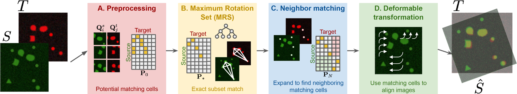
Schematic of the method (also see Alg. 1). A. We first filter the images to identify cells that potentially match $\left(\mathit{P}0\right)$, based on the cell shape and context. B. Maximum Rotation Set (MRS) algorithm then finds the exact subset match $\left(\mathit{P}*\right)$ using tree search and branch-and-bound routine. C. The pairs of cells from exact subset match are then expanded to include the neighbors $\left({\mathbf{P}}_{\mathbf{N}}\right)$ to solve an affine transformation. D. Based on phase correlation, deformable transformation is learned and applied to the source image.

A. Preprocessing (Fig 1A):

The first step is to obtain the potential cell match $\left({\mathbf{P}}_0\in \{\mathrm{0,1}{\}}^{M\times N}\right)$ based on their shapes and contexts. First, the point cloud descriptor of each cell $\left({\text{pcd}}_i^s,{\text{pcd}}_j^t\right)$ is obtained by downsampling the pixel location of all the segmented cells [14] $(s,t)$ in a small patch surrounding the target cell center $\left({\mathbf{Q}}_i^s,{\mathbf{Q}}_j^t\right)$. Then we use the 3D Iterative Closest Point (‘3D_ICP’) [15, 16] algorithm to find the potential transformation ${\mathbf{R}}_{i,j}^{\text{ICP}}$, for all $M\times N$ pairs of point cloud descriptors. After obtaining ${\mathbf{R}}_{i,j}^{\text{ICP }}$ between ${\text{pcd}}_i^s$ and ${\text{pcd}}_j^t$, Normalized Cross Correlation (‘NCC’) between ${\mathbf{Q}}_i^s$ and ${\mathbf{Q}}_j^t$ is used to quantify match quality. Since each patch may contain multiple cells, from the high-NCC pairs of patches, the final potential cell match ${\mathbf{P}}_0$ is calculated by examining cell co-occurrence in other patches of high-NCC cell pairs (‘CoOccur’).

B. Maximum Rotation Set (‘MRS’) (Fig 1B):

The goal of this step is to find the maximal subset of cells in $S$ and $T$ whose pairwise distances exactly match with each other (see triangulation in Fig. 1B). We cast this problem as the following subset selection objective function:

$$\begin{array}{l}\underset{P_{*}}{\text{max }}{1}^T{P}_{*}1,\\ \text{s}\text{.t. }{p}_{i,j}{p}_{i^{\prime },j^{\prime }}\left|d\left(x_i,x_{i^{\prime }}\right)-d\left(y_j,y_{j^{\prime }}\right)\right|<\gamma ,\hspace{1em}\mathbf{\text{rotation}}\\ P_{*}\mathbf{1}\le \mathbf{1},\hspace{1em}{\mathbf{\text{P}}}_{*}^T\mathbf{1}\le \mathbf{1},\hspace{1em}{P}_{*}\in {\left\{0,1\right\}}^{M\times N}\text{.}\hspace{1em}\mathbf{\text{permutation}}\end{array}$$ (1)

Here, ${\mathbf{P}}_{*}\in \{\mathrm{0,1}{\}}^{M\times N}$ captures which cells in $S$ and $T$ match. The rotation constraint ensures that all the pairs of matched cells in $S$ have the ‘same’ pair-wise distances with the pairs of matched cells in $T$. The permutation constraint makes sure that the matching is one-to-one.

We optimize Eq.(1) using a branch-and-bound algorithm by populating ${\mathbf{P}}_{*}$ one entry at a time, as detailed in Fig. 2. For each node $(i,j)$ in the search tree $\left(p_{i,j}=1\right)$, we first evaluate the objective function and constraints: (1) We compute the lower $\left(a\right)$ and upper $\left(b\right)$ bound of Eq.(1), which tell us the minimum and maximum number of cell matches we can have if we add $(i,j)$ to the match. (2) For rotation constraint, we check if the ordered pairwise distances within a set are no more than $\gamma$ away from the corresponding ordered pairwise distances within the other set. The pairwise distance matrices are shared between neighboring nodes except for one column and one row, and at each node we only need to update a linearly-increasing number of calculations to assess whether the set is still a rotation after adding a new pair of points. Therefore, $a$ and $b$ at each node can be updated efficiently using the results from previous nodes. (3) Permutation constraint is trivially satisfied because the search tree does not cover the same set of cells $(i,j)$ more than once. Thus after finding the maximal $a$ value in the search tree, and avoiding branches that have $b$ less than or equal to the current maximum $a$, we efficiently and globally optimize the maximum subset of exact matching cells.

Fig. 2.

Maximum Rotation Set (MRS) algorithm. One of the globally optimal paths is highlighted in yellow.

C. Neighboring cells matching (Fig.1C):

The exact subset match ${\mathbf{P}}_{*}$ gives us a locally rigid transformation of two images. However, due to shape mismatch and/or deformation, additional matching cells might have been excluded in the preprocessing step (Fig. 1A). So here we expand the covered region by including the neighboring cells of the exact subset match $\left({\mathbf{P}}_{\mathbf{N}}\right.$, ‘Neighbor_matching’). We do this by doing a final pass of 3D ICP [17, 15] using the locations of the cells in exact subset match ${\mathbf{P}}_{*}$ as an initializer. This outputs an updated transformation matrix ${\mathbf{R}}_{\mathbf{N}}$ and an expanded permutation matrix ${\mathbf{P}}_{\mathbf{N}}\in \{\mathrm{0, 1}{\}}^{M\times N}$ that captures additionally matched cells in $S$ and $T$.

D. Iterative deformable transformation (Fig.1D):

In the last step (‘Iterative_deformable_transform’), the tissue distortion is estimated. and the translations between pairs of patches are learned based on phase correlation [18]. Using the collection of local translation vectors, we obtain a global deformation field by smoothing it with a gaussian filter and iterating until convergence.

3. RESULTS

Evaluation metrics:

We used three different performance metrics: (1) Normalized cross correlation (NCC) measures image similarity independent of cell detections, (2) Target Registration Error (TRE) [8] measures the discrepancy of cell locations after matching, and (3) Number of cell matches to compare the performance with human-level alignment.

Specifically, TRE metric is defined as:

$${\text{TRE}}^{S,T}=\underset{c\in \left\{1,\dots N\right\}}{\text{median}}\left\{\frac{\parallel {\widehat{x}}_c-y_c\parallel }{\sqrt{d_1^{T^2}+d_2^{T^2}+d_3^{T^2}}}\right\},$$ (2)

where ${\hat{x}}_c$ is the predicted cell $\left(c\right)$ coordinates on transformed image $\hat{S},y_c$ is the corresponding cell’s coordinates in $T$. The denominator is the 3D diagonal of $T$.

Compared methods:

We considered the approaches presented in the recent “Automatic Non-rigid Histological Image Registration” (ANHIR) challenge [8] as the state-of-the-art methods for histology and microscopy image alignment. Of these methods, we focus on greedy [12, 13] because it is the backbone of the second-ranked method [19]. We also used greedy because is based on ANTs [20] and therefore it is able to operate on 3D images. Other methods in the ANHIR challenge were designed for 2D images of histology slides and were not applicable to our problem.

Simulated data evaluation and ablation study:

To generate simulation data, first we arbitrarily remove a certain number of random cells from the original image, using dilated masks of the segmented cells and flood-filling algorithm. Next, we transform the image with randomly sampled Euler angles and given scaling factors. Finally a randomly generated smooth vector field is applied to distort the image (Fig 3A).

Fig. 3. Method performance on simulation (blue background) and experimental (yellow background) data.

A: Simulation schematics. We started from the in vivo source image (orange) and generated realistic data that mimics the ex vivo target images (purple). B: We used three simulation settings to test our method’s performance against greedy [12, 13] based on normalized NCC (top, higher is better) and TRE (top, lower is better). C: Mouse hippocampal in vivo to ex vivo registration results, shown after the max-projection across z-planes. Matching cells can be seen in the overlaid yellow regions. D: Zoomed in registration results at three steps and corresponding NCCs with example cells from the exact subset match. E: Matched cell number comparison with manual alignment. F: Summary plot and table of the the comparison of ours (15–20 minutes), manual results (more than 2 hours), and greedy [12, 13] on the other datasets. Some matching cells are highlighted with magenta arrows.

We tested the method’s performance under three different simulation settings, as shown in the columns of Fig 3B. These are (1) the percentage of erased cells (green), (2) scaling factors (orange), and (3) added noise level (blue). When the parameters were fixed, they were chosen to take the middle values. We also show our method’s performance when ablating steps B, C and D in our pipeline. Our method is more robust to image distortion, and performs better in TRE and NCC than greedy (Fig 3B). We also found that greedy sometimes improves NCC but does not necessarily decrease TRE, suggesting that aligning purely based on image correlation may not be sufficient to address multimodality challenges.

Mouse hippocampus in vivo to ex vivo image alignment:

Next we applied our approach to experimental in vivo and ex vivo 3D images of hippocampal interneurons. Using the calcium indicator GCaMP, two modalities are taken from the same region using a two-photon imaging system and confocal microscopy. For the evaluation, no ground-truth cell locations were available for the experimental data, and the alignment found by greedy was not satisfactory, presumably because the problem is much more challenging. Therefore, we compared the matching cells detected by our method with those detected by manual matching (within $30\mu m$ distance) performed by an experimentalist.

The registration results are shown in Fig 3C–F. Panel C shows the overall registration results. Panel D shows the detailed registration results by ablating each step in our pipeline. Note that by using an exact subset match, we were able to find the general shifts of the images. Using neighboring cell location matches, we were able to learn the correct affine transformation as well as the tissue shrinkage scales (magenta boxes). However, to perfectly align the cells in the distorted tissue images (cyan box), the distortion pattern needs to be learned from deformable transformation. Our method identified additional cells beyond the manual registration method (panel E), and completed the tasks in substantially less time (15–20 minutes using 8 CPU cores and 32GB RAM, in contrast with manual registration which takes greater than 2 hours). We also compared our method with both the manual method and greedy [12, 13] on three other datasets and found that our method consistently performed well (panel F, $28.6\pm 18.8\%$ more matching cells than manual results with all four datasets tested).

Conclusion:

In this paper, we developed a method to find matching cells from multimodal microscopy images using an efficient branch-and-bound algorithm while pruning the search tree with initialization based on cell shapes and locations. Our approach outperforms the state-of-the-art histology alignment approaches [8, 12, 13], and is much faster than manual alignment, paving the way for increasing the throughput of multimodal experiments.

REFERENCES

- [1].Lovett-Barron Matthew, Chen Ritchie, Bradbury Susanna, Andalman Aaron S, Wagle Mahendra, Guo Su, and Deisseroth Karl, “Multiple convergent hypothalamus–brainstem circuits drive defensive behavior,” Nature neuroscience, vol. 23, no. 8, pp. 959–967, 2020. [DOI] [PMC free article] [PubMed] [Google Scholar]
- [2].Geiller Tristan, Vancura Bert, et al. , “Large-scale 3d two-photon imaging of molecularly identified ca1 interneuron dynamics in behaving mice,” Neuron, vol. 108, no. 5, pp. 968–983, 2020. [DOI] [PMC free article] [PubMed] [Google Scholar]
- [3].Anner Philip, Passecker Johannes, Klausberger Thomas, and Dorffner Georg, “Ca2+ imaging of neurons in freely moving rats with automatic post hoc histological identification,” Journal of Neuroscience Methods, vol. 341, pp. 108765, 2020. [DOI] [PubMed] [Google Scholar]
- [4].Gouwens Nathan W, Sorensen Staci A, Baftizadeh Fahimeh, Budzillo Agata, Lee Brian R, Jarsky Tim, Alfiler Lauren, Baker Katherine, Barkan Eliza, Berry Kyla, et al. , “Integrated morphoelectric and transcriptomic classification of cortical gabaergic cells,” Cell, vol. 183, no. 4, pp. 935–953, 2020. [DOI] [PMC free article] [PubMed] [Google Scholar]
- [5].Xu Shengjin, Yang Hui, Menon Vilas, Lemire Andrew L, Wang Lihua, Henry Fredrick E, Turaga Srinivas C, and Sternson Scott M, “Behavioral state coding by molecularly defined paraventricular hypothalamic cell type ensembles,” Science, vol. 370, no. 6514, pp. eabb2494, 2020. [DOI] [PMC free article] [PubMed] [Google Scholar]
- [6].Bugeon Stephane, Duffield Joshua, Dipoppa Mario, Ritoux Anne, Prankerd Isabelle, Nicoloutsopoulos Dimitris, Orme David, Shinn Maxwell, Peng Han, Forrest Hamish, et al. , “A transcriptomic axis predicts state modulation of cortical interneurons,” bioRxiv, 2021. [DOI] [PMC free article] [PubMed] [Google Scholar]
- [7].Condylis Cameron, Ghanbari Abed, Manjrekar Nikita, Bistrong Karina, Yao Shenqin, Yao Zizhen, Nguyen Thuc Nghi, Zeng Hongkui, Tasic Bosiljka, and Chen Jerry L, “Dense functional and molecular readout of a circuit hub in sensory cortex,” Science, vol. 375, no. 6576, pp. eabl5981, 2022. [DOI] [PMC free article] [PubMed] [Google Scholar]
- [8].Borovec Jiří, Kybic Jan, et al. , “Anhir: automatic non-rigid histological image registration challenge,” IEEE transactions on medical imaging, vol. 39, no. 10, pp. 3042–3052, 2020. [DOI] [PMC free article] [PubMed] [Google Scholar]
- [9].Wodzinski Marek and Müller Henning, “Deephistreg: Unsupervised deep learning registration framework for differently stained histology samples,” Computer Methods and Programs in Biomedicine, vol. 198, pp. 105799, 2021. [DOI] [PubMed] [Google Scholar]
- [10].Ko Ho, Hofer Sonja B, Pichler Bruno, Buchanan Katherine A, Sjöström P Jesper, and Mrsic-Flogel Thomas D, “Functional specificity of local synaptic connections in neocortical networks,” Nature, vol. 473, no. 7345, pp. 87–91, 2011. [DOI] [PMC free article] [PubMed] [Google Scholar]
- [11].von Buchholtz Lars J, Ghitani Nima, Lam Ruby M, Licholai Julia A, Chesler Alexander T, and Ryba Nicholas JP, “Decoding cellular mechanisms for mechanosensory discrimination,” Neuron, vol. 109, no. 2, pp. 285–298, 2021. [DOI] [PMC free article] [PubMed] [Google Scholar]
- [12].Yushkevich Paul A, Pluta John, Wang Hongzhi, Wisse Laura EM Das Sandhitsu, and Wolk David, “Icp-174: Fast automatic segmentation of hippocampal subfields and medial temporal lobe subregions in 3 tesla and 7 tesla t2-weighted mri,” Alzheimer’s & Dementia, vol. 12, pp. P126–P127, 2016. [Google Scholar]
- [13].Yushkevich Paul, “greedy (fast deformable registration for 3d medical images),” https://github.com/pyushkevich/greedy, 2014.
- [14].Stringer Carsen, Wang Tim, Michaelos Michalis, and Pachitariu Marius, “Cellpose: a generalist algorithm for cellular segmentation,” Nature Methods, vol. 18, no. 1, pp. 100–106, 2021. [DOI] [PubMed] [Google Scholar]
- [15].Besl Paul J and McKay Neil D, “Method for registration of 3-d shapes,” in Sensor fusion IV: control paradigms and data structures. International Society for Optics and Photonics, 1992, vol. 1611, pp. 586–606. [Google Scholar]
- [16].Chen Yang and Medioni Gérard, “Object modelling by registration of multiple range images,” Image and vision computing, vol. 10, no. 3, pp. 145–155, 1992. [Google Scholar]
- [17].Wahba Grace, “A least squares estimate of satellite attitude,” SIAM review, vol. 7, no. 3, pp. 409–409, 1965. [Google Scholar]
- [18].Pnevmatikakis Eftychios A and Giovannucci Andrea, “Normcorre: An online algorithm for piecewise rigid motion correction of calcium imaging data,” Journal of neuroscience methods, vol. 291, pp. 83–94, 2017. [DOI] [PubMed] [Google Scholar]
- [19].Venet Ludovic, Pati Sarthak, Yushkevich Paul, and Bakas Spyridon, “Accurate and robust alignment of variable-stained histologic images using a general-purpose greedy diffeomorphic registration tool,” arXiv preprint arXiv:1904.11929, 2019. [Google Scholar]
- [20].Avants Brian B, Epstein Charles L, Grossman Murray, and Gee James C, “Symmetric diffeomorphic image registration with cross-correlation: evaluating automated labeling of elderly and neurodegenerative brain,” Medical image analysis, vol. 12, no. 1, pp. 26–41, 2008. [DOI] [PMC free article] [PubMed] [Google Scholar]