Control-independent mosaic single nucleotide variant detection with DeepMosaic

Abstract

Mosaic variants (MVs) reflect mutagenic processes during embryonic development and environmental exposure, accumulate with aging, and underlying diseases such as cancer and autism. The detection of noncancer MVs has been computationally challenging due to the sparse representation of non-clonally expanded MVs. Here we present DeepMosaic, combining an image-based visualization module for single nucleotide MVs, and a convolutional neural networks-based classification module for control-independent MV detection. DeepMosaic was trained on 180,000 simulated or experimentally-assessed MVs and was benchmarked on 619,740 simulated MVs, and 530 independent biologically tested MVs from 16 WGS, and 181 WES. DeepMosaic achieved higher accuracy compared with existing methods on biological data, with a sensitivity of 0.78, specificity of 0.83, and positive predictive value of 0.96 on noncancer WGS, as well as doubling the validation rate over prior best-practice methods on noncancer WES data (0.43 vs 0.18). DeepMosaic represents an accurate MV classifier for noncancer samples that can be implemented as an alternative or complement to existing methods.

Postzygotic mosaicism describes a phenomenon whereby cells arising from one zygote harbor distinguishing genomic variants^{1, 2}. MVs can act as recorders of embryonic development, cellular lineage, and environmental exposure. They accumulate with aging^{2, 3} and are implicated in over 200 noncancerous disorders^{4, 5}. Collectively, MVs are estimated to contribute to 5-10% of the ‘missing genetic heritability’ in more than 100 human disorders^{4, 6–8}.

Compared with the higher allelic fractions (AF) of 5-10% found in cancer or pre-cancerous mosaic conditions, AFs found in non-clonal disorders, or neutral variants used for lineage studies, are frequently an order of magnitude lower. Existing methods like MuTect2⁹ and Strelka2¹⁰, however, are based on classic statistical models, using heuristic filters that are often optimized for higher AF MVs seen in cancer. Similarly, because of their conceptual origin in cancer, most existing programs, including the recent NeuSomatic¹¹, also require matched ‘noncancer’ control samples. This can be problematic when mutations are present across different tissues (‘tissue shared’ mosaicism), or when only one sample is available.

Recent methods that aim to overcome these limitations in noncancer MV detection, MosaicHunter¹², and MosaicForecast¹³, are based on conceptually similar use of features extracted from raw data, rather than the sequence and alignment themselves, or replace heuristic filters with traditional machine-learning methods. While these are useful proxies, they represent a limited window into the sheer wealth of information contained in raw sequencing data. Furthermore, performance on whole-exome sequencing (WES) data is limited due to the intrinsically biased experimental nature of exome capture^{13, 14}. To address these limitations, researchers often resort to visual inspection of raw sequence alignment in a genome browser, a so-called ‘pileup’, to distinguish artifacts from true positive MVs¹⁵. This is a laborious and low-throughput process that allows spot checking, but cannot be implemented on a large scale for putative MV lists generated from programs like MuTect2 or GATK Haplotypecaller using ‘ploidy’ setting of 50 ¹⁶ often numbering in thousands.

Image-based representation of raw sequencing reads and the application of deep convolutional neural networks (CNNs) represent a potential solution for these limitations for non-MV detection. An example approach like DeepVariant¹¹ was designed and trained for detecting only heterozygous or homozygous single nucleotide variants (SNVs) from direct representation of aligned reads. DeepVariant, however, cannot be used for noncancer MV detection. Here, we introduce DeepMosaic, comprised of two modules: a visualization module for image-based representation of SNVs separating reference and alternative supporting reads, as input for a convolutional neural network (CNN)-based classification module for MV detection. Nine different biological and computationally simulated datasets were used to train and benchmark DeepMosaic. Finally, large-scale deep amplicon sequencing (Methods) provided an orthogonal experimentally validated set of DeepMosaic-detected variants and allowed for direct comparison with other state-of-the-art methods.

To automatically generate a useful visual representation similar to a browser snapshot, we developed the visualization module of DeepMosaic (DeepMosaic-VM, Fig. 1a–d). The input for this visualization is short-read sequencing data, processed with a GATK current best-practice pipeline (insertion/deletion, or INDEL, realignment, followed by base quality score recalibration). DeepMosaic-VM exports this data into an ‘RGB’ image, representing a pileup at each genomic position (Method). In contrast to a regular browser snapshot used in DeepVariant, DeepMosaic encodes sequences as different intensities within one channel and uses other channels for base quality and strand orientation. DeepMosaic further separates the pileups into ‘ref’ reads and ‘alt’ reads based on the reference genome information (Fig. 1a–d). This improved pileup visualization allows the assessment of mosaicism at a glance for humans, and converts the biological variant detection problem into an edge- and shape-detection problem, which is more suitable for image-based classification by CNN models.

Fig. 1|. Image representation, model training strategies, and framework of DeepMosaic.

a, DeepMosaic-VM: Composite RGB image representation of sequenced reads separated into “Ref” - reads supporting the reference allele; or “Alts’’ - reads supporting alternative alleles; each outlined in yellow. b, Red channel of the compound image contains base information from the BAM file. “D” - deletion; “A” – Adenine; “C” – cytosine; “G” – guanine; “T” – thymine; “N” – low-quality base. Yellow box: Var: candidate position, centered in the image. c, Green channel: base quality information. Note that channel intensity was modulated in this example for better visualization. d, Blue channel: strand information (i.e. forward or reverse). e, Model training, model selection, and overall benchmark strategy for DeepMosaic-CM (Methods and Supplementary Fig. 1). Ten different convolutional neural network models were trained on 180,000 experimentally validated positive and negative biological variants from 29 WGS data from 6 individuals sequenced at 100x^{17, 18} (BioData1), as well as simulated data with different AFs (SimData1) resampled to a different depth. Models were evaluated based upon an independent gold-standard biological dataset from the 250x WGS data of the Reference Tissue Project of the Brain Somatic Mosaicism Network¹⁶ (BioData2) as well as an independent 300x WGS dataset from the Brain Somatic Mosaicism Network Capstone project¹⁹ (Biodata3). DeepMosaic was further benchmarked on 16 independent biological datasets from 200x WGS data²⁸ (BioData4), on 181 independently generated 300x noncancer WES data (BioData5), 2430 TCGA-MC3 WES samples (BioData6), as well as 619,740 independently simulated variants (SimData2 and SimData3). Deep amplicon sequencing was carried out as an independent evaluation of variants detected by different software (Supplement Table 1). f, Application of DeepMosaic-CM in practice. Input images are generated from the candidate variants. 16 convolutional layers extracted information from input images. Population genomic features were assembled for the final output. Images of positive and negative variants are shown as examples. Conv: convolutional layers; MBConv: mobile convolutional layers.

The classification module of DeepMosaic (DeepMosaic-CM) is based on CNN transfer learning for MVs. We trained 10 different CNN models with more than 180,000 image-based representations from both true-positive and true-negative biological variants derived from several previously published high-quality public datasets with orthogonal experimental validations by amplicon sequencing or droplet digital PCR techniques^17–19. To subsidize the requirement for CNN training, we included ~50% computationally simulated reads with spiked-in MVs (employing Illumina HiSeq error models) across a range of AFs and depths (Fig. 1e, Methods, and Supplementary Fig. 1a–b). This training dataset (BioData1 and SimData1) was aimed to train a model with optimal performance on noncancer MV detection. To ensure performance in ‘real-world’ settings, we matched the distribution of AFs in the training set with experimentally determined AFs (Supplementary Fig. 1c). In addition, a range of expected technical artifacts, including false-positive variants with multiple alternative alleles, false-positive variants located near homopolymers >5 bp or on the edge of di-nucleotide repeats, and variants that are detected as alignment artifacts after the validation experiments^{17, 18}, were manually curated and labeled as negative in the training set to represent expected pitfalls that often result in false positive noncancer MVs for other programs (Supplementary Fig. 1d).

To further expand training across a range of different read depths, the biological training data were also up- and down-sampled to obtain data at read depths ranging from 30x to 500x (Supplementary Fig. 1e), covering the range of the most commonly used WGS and WES read depths in current clinical and scientific settings. In addition to the output from DeepMosaic-VM, we further incorporated population genomic and sequence features (e.g. population allele frequency from population study, genomic complexity from field-acceptable database, the ratio of read depth by experimental design), which are not easily represented in an image, as input for the classifier (Fig. 1f). Depth ratios were calculated from the expected depth and used to exclude false-positive detections from potential copy number variations (CNVs) or aneuploidies. gnomAD population allelic frequencies were used to exclude common variants²⁰. Segmental duplication and repeat masker regions were used to exclude 24% of the genome consisting of low-complexity regions.

Ten different CNN architectures were trained on the 180,000 variants described above. The CNN models included Inception-v3 ²¹, which was re-trained and used by DeepVariant; Deep Residual Network²² (Resnet) which was re-trained and used in the control-dependent caller NeuSomatic; Densenet²³, and 7 different builds of EfficientNet²⁴, to optimize performance on rapid image classification (details were documented in Methods, network structure and dimension of convolutional layers are provided in Supplementary Fig. 2a). Each model was trained with 5 to 15 epochs to optimize the hyper-parameters until training accuracies plateaued (>0.90).

To compare the performance of post-training models and to contrast models trained with distinct datasets, we employed an independent gold-standard validation dataset of ~400 MVs from one gold-standard brain sample generated by the Brain Somatic Mosaicism Network¹⁶ (BioData2, Methods) and another amplicon-validated dataset from 18 samples from a publicly available dataset we recently published¹⁹ (BioData3, Methods). On these, EfficientNet-b4 showed the highest accuracy, Matthews’s correlation coefficient, and true positive rate when trained for 6 epochs (Supplementary Fig. 2b). We thus selected this as the default model of DeepMosaic-CM (Fig. 1f). Additional EfficientNet-b4 models trained on the 1:1 mixture of biological data and simulated data showed similar performance compared with biological data only training set but much higher specificity compared with models trained only on simulated data (Supplementary Fig. 2c).

To uncover the information prioritized by the selected default model, we used a gradient visualization technique with guided backpropagation²⁵ to highlight the pixels guiding classification decisions (Supplementary Fig. 3). The results suggested that the algorithm not only recognized the edges for reference and alternative alleles, but also integrated additional available information, such as insertion/deletions, overall base qualities, alignment artifacts, and other features, which may not be extracted by digested feature-based methods.

We evaluated the performance of DeepMosaic using 20,265 variants from the training data that were hidden from model training and selection. The receiver operating characteristic (ROC) curve and precision-recall curves on the hidden validation dataset showed >0.99 area under the curve for a range of coverages (30x ~500x, Supplementary Fig. 4a and 4b) across a range of AFs (Supplementary Fig. 4c and 4d), demonstrating good sensitivity and specificity.

Next, we benchmarked DeepMosaic’s performance relative to other detection software, using data generated from two distinct sequencing error models to test for its utility on general sequencing data. We compared the performance of DeepMosaic with the widely used MuTect2 (paired mode) and Strelka2 (somatic mode) followed by heuristic filters, MosaicHunter (single mode), and MosaicForecast (Methods). We generated two additional computationally simulated datasets of 439,200 and 180,540 positions based on the error model of a different Illumina sequencer with similar methods as the training set (NovaSeq, SimData2, Methods) or a similar ratio of true positive and true negative labels as real biological data¹⁹ by replacing reads from the ‘Genome in a Bottle’ sample HG002 (NA24345, SimData3, Methods)^{26, 27}, with AF ranges from 1% to 25%, and depth ranges from 50x to 500x. MuTect2 paired mode and Strelka2 somatic mode used simulated mutated samples as “tumor” and simulated reference or original HG002 samples as “normal” for their paired modes. DeepMosaic showed equal or better performance than all other methods tested, especially for low AF variants (Fig. 2 and Supplementary Fig. 5), noticeably, even for low read depth data (50x); and it performed better than methods that use the additional information from paired samples. Overall DeepMosaic showed a 1.5-3 fold increased detection sensitivity for AFs under 3% compared with other methods, with comparable specificity (Fig 2). This is likely because our models integrate additional genomic sequence and quality information from the original BAM file and are capable of distinguishing MVs from false-positive variants resulting from different sequencing errors.

Fig. 2|. DeepMosaic performance on simulated benchmark variants.

a, Benchmark test on 180,540 genomic positions (SimData3) generated by replacing reads from biological data with simulated MVs. DeepMosaic showed higher accuracy, F1 score, MCC (Matthews correlation coefficient), sensitivity, and comparable specificity compared with widely accepted methods for mosaic variant detection, specificity of all callers are close to 1. b, Sensitivity of DeepMosaic and other mosaic callers on SimData3 at simulated read depths and AFs. DeepMosaic performed equally well or better than other tested methods, especially at lower read depths and lower expected AFs. Variant-stabilized square-root transformation was used for visualization purposes.

To exclude limitations resulting from benchmarking with simulated data and demonstrate that models trained on PCR-amplified libraries are also useful for PCR-free sequencing libraries, we extended benchmarking to biological data. We performed the same comparison on the previously published 200x WGS dataset with 16 samples (blood and sperm) from 8 healthy individuals^{7, 28} (BioData4). Paired methods compared two samples from the same individual, and control-independent samples used a published dataset of a panel of normals⁷. Variants detected by MuTect2 (paired mode), Strelka2 (somatic mode), and MosaicHunter (single mode) were subjected to a series of published heuristic filters^{7, 28}. As we had access to the biological samples, we also performed orthogonal validation, using deep amplicon sequencing of 239 MVs with a representative AF distribution compared to the complete candidate variant list (Methods, Fig. 3a and 3b, Supplementary Table 1).

Fig. 3|. DeepMosaic performance validated on biological data.

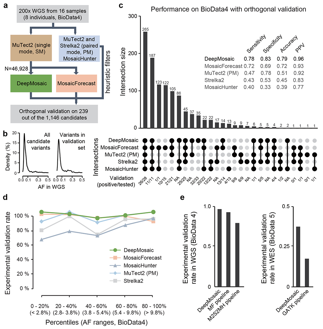
a, DeepMosaic and other mosaic variant detection methods were applied to 200x whole-genome sequencing data from 16 samples, which were not used in the training or validation stage for any of the listed methods (BioData4). Raw variant lists were either obtained by comparing samples using a panel-of-normal⁷ strategy with MuTect2 single mode, between different samples from the same individual using MuTect2 paired mode or Strelka2 somatic mode or detected directly without control with MosaicHunter single mode with heuristic filters²⁸. A total of 46,928 candidate variants from MuTect2 single mode were analyzed by DeepMosaic and MosaicForecast. Orthogonal validation with deep amplicon sequencing was carried out on a total of 239 variants out of the 1146 candidates called by at least one method. b, Distribution of AFs of the whole candidate mosaic variant list and the 239 experimentally quantified variants. c, Comparison of validation results between different mosaic variant calling methods, ‘UpSet’ plot shows the intersection of different mosaic detection methods and the validation result of each category. Variants identified by DeepMosaic showed high sensitivity and specificity to biological data. d, Comparison of validation rate in different AF range percentage bins of variants. DeepMosaic showed the highest validation rate at a range of AFs, approximately 48 experimentally validated variants are shown in each AF bin. e, Comparision of experimental validation rate of DeepMosaic on WGS (BioData4) and WES (BioData5) outperforms other computational pipelines.

As expected from the test of the computationally generated data, DeepMosaic showed a high sensitivity (0.78), specificity (0.83), accuracy (0.79), and overall validation rate (96.3%, 158/164) among all 5 methods (Fig. 3c), demonstrating that DeepMosaic, trained on PCR-amplified biological data and simulated data, can accurately classify PCR-free biological data. Of the 819 WGS MVs detectable by DeepMosaic, 21.0% (172/819, 33/34 experimentally validated as positive) were overlooked by MosaicForecast, 30.1% (247/819, 96/98 validated) by MosaicHunter, 26.7% (219/819, 90/94 validated) by Strelka2 (somatic mode) with heuristic filters, and 42.9% (351/819, 81/85 validated) by MuTect2 (paired mode) with heuristic filters²⁸. DeepMosaic also accurately detected variants with relatively low AF and outperformed other methods across most of the AF bins (Fig. 3d). We additionally tested the performance of NeuSomatic on the same dataset, and it showed higher specificity (0.92) but much lower sensitivity (0.33) on the orthogonally validated dataset (Supplementary Fig. 6). 49.9% DeepMosaic variants (409/819, 99/105 validated) were missed by NeuSomatic, indicating that neural networks trained on cancer data might underperform on a noncancer biological dataset.

In current practice, researchers often combine multiple programs in one variant detection pipeline to detect different categories of MVs^{7, 28, 29}. We thus further compared DeepMosaic with different WGS pipelines used in recent publications, using data from 200x WGS of the 16 samples²⁸: 1] With the MosaicForecast pipeline¹³, which uses MuTect2 single mode (each sample compared with the publicly available panel of normal) as input; 2] With what we recently published as the M2S2MH pipeline ²⁸, combining MuTect2 paired mode (i.e. compared between different samples from the same individual), Strelka2 somatic mode and MosaicHunter single mode followed by a series of heuristic filters (Supplementary Fig. 7a). Of the 819 MVs identified by DeepMosaic, 79.0% (647/819, 125/130 validated) overlapped with MosaicForecast and 68.4% (560/819, 87/91 validated) overlapped with M2S2MH. In contrast, 21.0% (172/819, 33/34 validated) were undetected by MosaicForecast, and 33.0% (271/819, 71/73 validated) were overlooked by M2S2MH. These variants, uniquely detected by DeepMosaic, all showed validation rates> 95% (Supplementary Fig. 7b–d), demonstrating the accurate detection of a considerable number of variants undetectable by widely used methods.

To test the performance of DeepMosaic on data widely curated clinically, we compared detection sensitivity for genome samples with standard WGS read depth, by down-sampling blood-derived data from a 70-year-old healthy individual, in whose blood we observed the highest number of mosaic variants (due to clonal hematopoiesis²⁸). As all programs had high validation on this sample at 200x, the recovery rate was used to distinguish the ability of different programs to detect clonal hematopoiesis variants. DeepMosaic showed a similar recovery in the down-sampled data (Supplementary Fig. 8) as M2S2MH and slightly outperformed MosaicForecast at 100x and 150x. We found that the performance of DeepMosaic was not substantially influenced by the read depth according to the down-sampling benchmark on biological data.

To understand whether different WGS pipelines had unique strengths or weaknesses, we separated all the detected variants into 7 groups (G1-G7) based on sharing between different pipelines (Supplementary Fig. 8a). DeepMosaic specific variants showed similar base substitution features compared with other methods (Supplementary Fig. 8b). Similar to the computationally derived data, we found that DeepMosaic recovered additional low AF MVs with high accuracy (validation rate 95%, Supplementary Fig. 8c). Finally, we summarized the genomic features of variants detected by DeepMosaic and other pipelines. All caller groups reported similar ratios of intergenic and intronic variants (Supplementary Fig. 9a). Analysis of other genomic features showed DeepMosaic-specific variants (G1) expressed consistency with other groups (Supplementary Fig. 9b), reflecting that the low-fraction variants detectable only by DeepMosaic did not represent technical artifacts. Further detailed SBS signature analyses with a larger number of variants will shed light on genetic mechanisms detected by DeepMosaic and other callers at different AF.

Compared to WGS, the selection of exonic regions in WES is prone to introducing capture bias and other artifacts, which can impact MV detection, often exhibiting relatively low detection rates and high false-positive rates¹⁴. Furthermore, methods like MosaicForecast do not explicitly support WES¹³. As the image representation of WES—unlike the classical feature extraction methods—is expected to be similar to WGS, we postulated that DeepMosaic, even as currently trained on genome data, could perform satisfactorily on WES data as well. Thus, we benchmarked DeepMosaic on our recent noncancer WES dataset. Of 181 samples from 101 individuals who underwent 300x WES (BioData5, Methods, Supplementary Fig. 10a and 10b), candidate MVs were detected by DeepMosaic and the BSMN best-practice pipeline¹⁶. Experimental validation on 291 of the 585 candidate variants showed a higher validation rate for DeepMosaic (43.1%) compared with the best-practice pipeline (17.6%, Fig. 3e and Supplementary Table 2). DeepMosaic also consistently demonstrated high specificity (0.86) and accuracy (0.78), with compromised sensitivity (0.43) likely due to differences in the nature of exonic and genomic sequencing. Thus, DeepMosaic has the ability to complement and potentially improve upon existing pipelines on large-scale existing noncancer WES data.

Compared to noncancer MVs, the clonal expansion of cancer-related MVs will result in a much higher portion of cancer MVs in the genome, and different mutation features for tools to recognize. NeuSomatic was trained on cancer samples and demonstrated lower sensitivity on noncancer MVs (Supplementary Fig. 6). We expect similar performance for DeepMosaic for cancer samples, and thus systematically estimated the performance of DeepMosaic, with its current models, on cancer WES data. We re-processed 2430 WES samples from the TCGA-MC3 data collection (BioData6 and Methods), employed DeepMosaic, and compared the result with 5 other callers (MuSE³⁰, MuTect⁹, SomaticSniper³¹, VarScan2 ³², and Radia³³) provided in the original publications³⁴. Benchmarked by the gold-standard dataset³⁴, DeepMosaic demonstrated high specificity (0.97) and accuracy (0.77), similar to noncancer WES and WGS. Due to the different nature of somatic mutations described above, however, the sensitivity was lower (0.08, Supplementary Table 3 and Supplementary Table 4). We found that some variants defined as technical artifacts in the DeepMosaic training set, for example, 24% of variants with allelic fractions higher than 0.5 (674175 of 2814168 total variants), variants with multiple alternative alleles, and/or with copy number alternations or aneuploidies, were defined as true positive in tumor samples. As such, we do not recommend the use of DeepMosaic for cancer in its current form, unless further training sets are used to optimize the detection of these mutation types.

While the cancer WES datasets were not suitable for DeepMosaic, they were suitable for the estimation of computational resources. We further estimated the computational resources for DeepMosaic based on 1215 WES and 48 WGS datasets, DeepMosaic consumed an average of 1403.8 (range 9.1-50168.9) seconds on one WES sample and 22718.2 (range 6565.8 – 60800.0) seconds for a 300x genome, an average of 1.3Gb (range 0.9Gb – 1.8Gb) maximum memory for an exome and an average of 1.2Gb (range 1.1Gb – 1.3Gb) for a genome, which could be accelerated by more CPU nodes or using GPU nodes (Supplementary Table 5, Supplementary Fig. 10c and 10d).

DeepMosaic detects noncancer mosaic SNVs from short-read sequencing data and does not require a matched control sample. Compared with NeuSomatic which compresses all the bases in a genomic position into 10 features³⁵, DeepMosaic-VM provides a complete representation of information present in the BAM file and showed higher sensitivity on noncancer MVs. Compared with other re-coding methods like DeepVariant¹¹, DeepMosaic-CM can distinguish between MVs and other genotypes. DeepMosaic-VM can be applied as an independent variant visualization tool for users’ convenience. To further improve accuracy, DeepMosaic integrates four genomic features and population information absent in the raw BAM files.

Both biological and simulated data showed that DeepMosaic has the potential to identify MVs at relatively high sensitivity and accuracy for WGS at depths as low as 50x. For the past 10-15 years, hundreds of thousands of WGS datasets from clinical, commercial, or research labs have been generated at relatively low depth, but most have not been subjected to unbiased mosaicism detection due to the lack of sufficiently sensitive methods. DeepMosaic could enable a genome-level unbiased MV detection that requires only conventional sequencing data. For instance, clonal hematopoiesis without a known driver mutation is reported³⁶ but can be difficult to detect because of technical limitations induced by noise and lower supporting read counts³⁷.

By using a training set comprising representative technical artifacts such as homopolymers and truncated reads, DeepMosaic acquired the power to distinguish biologically true positive from false positive MVs. These might have otherwise been filtered out by rule-based methods like MosaicHunter¹² or MosaicForecast¹³. We demonstrated that training the models on a mixture of ~1:1 simulated and biological data did not adversely affect performance on an independent biological evaluation set. We also demonstrated that DeepMosaic worked well for various Illumina short-read sequencing platforms applying different library preparation strategies (PCR-amplified and PCR-free).

Although the EfficientNet-b4 model performed best, we provide all pre-trained CNN models (Densenet, EfficientNet, Inception-v3, and Resnet) on GitHub. DeepMosaic users can prepare their own data with labeled genotypes for training, generate data-specific, personalized models, test other potential factors influencing detection sensitivity such as the ratio of positive: negative labels, and increase the detection specificity on specialized data sets. For instance, homopolymers and tandem repeats are increasingly recognized in disease and development, but, because of the limited training data, are currently not detected with DeepMosaic; however, users could retrain with such specialized datasets. Likewise, although detecting MVs from WES can be challenging, DeepMosaic outperformed the existing best-practice pipeline. We propose that further training on large-scale experimentally-validated WES data could further improve performance.

While we propose DeepMosaic as a tool for MV detection in WGS and WES, it is not designed to detect mosaic INDELs and mosaic repetitive variants, regions known to be fraught with errors, nor is DeepMosaic, in its current form, suitable for cancer samples. In practice, MosaicForecast can detect mosaic INDEL variants with reasonable accuracy, while M2S2MH has good performance for tissue-specific variants due to the inclusion of additional information from the “normal” comparison sample. And methods such as MuTect2 paired mode showed a higher sensitivity for cancer samples. Thus, different methods complement one another and should be selected for the purpose.

Despite the features from image representation and a neural network-based variant classifier, DeepMosaic can reproducibly identify the majority (~70%) of WGS MVs detectable by conventional methods. This unique architecture results in higher sensitivity, and the detection of variants with relatively lower AF, both in simulated and experimentally derived, and orthogonally validated data. DeepMosaic shows a drop of sensitivity at higher AF, likely due to the inclusion of depth ratio, which helps to avoid false-positive calls from CNV. DeepMosaic showed consistently high accuracy in noncancer WGS and WES data (Supplementary Table 4) and thus is suitable for high-specificity variant detection. Nevertheless, the higher accuracy at lower AFs should make it a good complement to other methods.

Population allele frequencies used in this study also rely on a matched ancestry background to avoid population stratification. Annotations such as gene names, variant functional annotations, gnomAD allelic frequency, homopolymer, and dinucleotide repeat annotation, as well as segmental duplication and UCSC repeat masker regions are provided in the final output to facilitate customization, as described at the GitHub homepage of DeepMosaic (https://github.com/Virginiaxu/DeepMosaic). Finally, apart from MuTect2 single mode, DeepMosaic can also process WGS and WES variant lists generated by multiple methods such as the GATK HaplotypeCaller with “ploidy” 50 or 100¹⁶. Thus, DeepMosaic can be used directly as is or can be customized to the needs of the end-users, providing an adaptable MV detection workflow.

Methods

Visualization of MVs

Visualization of mosaic variants was based on Python (v3.7.81) packages Pysam (v0.11.2.2, https://github.com/pysam-developers/pysam) and NumPy (v1.16.2, https://numpy.org/), The input for this visualization is short-read sequencing data in the format of a BAM file, processed with a GATK (v3.8.1) best-practice pipeline (with insertion/deletion, or INDEL, realignment, followed by base quality score recalibration). Inspired by DeepVariant¹¹, DeepMosaic-VM exports this data into an ‘RGB’ image, representing a pileup at each genomic position, as well as generating a NumPy object for the classification module. In contrast to presenting scattered reads by DeepVariant, DeepMosaic encodes separated sequences piling up into ‘ref’ reads and ‘alt’ reads based on the reference genome information. This improves pileup visualization and allows the assessment of mosaicism at a glance for humans, and converted the biological variant detection problem into an edge- and shape-detection problem, which is more suitable for image-based classification by convolutional neural network models (https://github.com/Virginiaxu/DeepMosaic/blob/master/deepmosaic/featureExtraction.py).

Curation of training and benchmark data

SimData1:

For the initial training procedure, 10,000 variants were randomly generated on chromosome 22 to get the list of alternative bases. Pysim³⁸ was then used to simulate paired-end sequencing reads with random errors generated from the Illumina HiSeq sequencer error model. Alternative reads were generated by replacing the genomic bases with the alternative bases in the list, with the same error model. Alternative and reference reads were randomly mixed to generate an alternative AF of 0, 1, 2, 3, 4, 5, 10, 15, 20, 25, and 50%. The data were randomly sampled for a targeted depth of 30, 50, 100, 120, 150, 200, 250, 300, 400, and 500x. FASTQ files were aligned to the GRCh37d5 human reference genome with BWA (v0.7.17) mem command. Aligned data were processed by GATK (v3.8.1) and Picard (v2.18.27) for marking duplicates, sorting, INDEL realignment, base quality recalibration, and germline variant calling. The up- and down-sampling expanded this dataset into a pool of 990,000 different variants. Depth ratios were calculated as defined. To avoid the situation that randomly generated mutations fall on a common SNP position in the genome, which would bias the training and benchmarking, gnomAD allele frequencies were randomly assigned from 0 to 0.001 for simulated mosaic positive and from 0 to 1 for simulated negative variants, which were established as homozygous or heterozygous.

SimData2:

To compare the performance of DeepMosaic and other software to detect mosaicism on simulated data, we randomly generated another simulation dataset, with the following modifications: 1] only 7610 variants on the non-repetitive region of chromosome 22 were considered true positive genomic positions; 2] random errors were generated from the Illumina NovaSeq sequencer error model. 3] Data was randomly down-sampled and up-sampled for a targeted depth of 50, 100, 200, 300, 400, and 500x. A total of 439,200 different variants were generated. FASTQ files were aligned and processed with BWA (v0.7.17), SAMtools (v1.9), and Picard (v2.18.27). The data were subjected to DeepMosaic as well as MuTect2 (GATK v4.0.4, both paired mode and single mode), Strelka2 (v2.9.2), MosaicHunter (v1.0.0), and MosaicForecast (v8-13-2019) with different models trained for different read depth (250x model for depth≥300x).

SimData3:

We further generated another simulation dataset in a way that was fundamentally different from the training data with a positive: negative ratio similar to real data¹⁹ to compare the performance of DeepMosaic and other software for the detection of mosaic variants. We selected 30,090 genomic positions with reference homozygous genotype from a different genomic region (the entire Chromosome 1) of the whole-genome deep sequences from the ‘Genome In a Bottle’ sample HG002 (NA24345)²⁷. The genomic positions from the 30,090 positions were genotyped as homozygous and fulfilled additional criteria 1] zero alternative bases in the raw sequencing data; 2] no detectable insertions/deletions in the position of interest; 3] have a genomic distance of at least 1000 bases between each other. On this clear background, 15,471 of them were labeled as “true negative“ with reference homozygous genotype, and 6868 were labeled as “true positive” mosaic variants with expected alternative AF 0.01, 0.02, 0.03, 0.04, 0.05, 0.10, 0.15, 0.20, and 0.25 (on average 763 variants for each genotype); 7751 were labeled as “true negative” heterozygous variants with alternative AF 0.50; the latest version of a different software BAMSurgeon (updated 24 Dec 2020) was used to generate this simulation dataset and retain the sequencing errors from the original biological samples. The original bam file was first up-sampled, and alternative reads were replaced to generate the expected AF, mapped back to the genome, and merged back to the bam file, according to the software manual²⁶. Bam files with and without simulated data were downsampled to 500x, 400x, 300x, 200x, 100x, and 50x. The data were subjected to DeepMosaic as well as MuTect2 (GATK v4.0.4, both paired mode, and single mode), Strelka2 (v2.9.2), MosaicHunter (v1.0.0), and MosaicForecast (v8-13-2019) with different models trained for different read depth (250x model for depth≥300x), the performance of the 180,540 points were evaluated.

BioData1:

Variant information and raw sequencing read from 80-120x PCR-amplified PE-150 WGS data of 29 samples from 6 normal individuals were extracted from published data^{17, 18} on SRA (SRP028833, SRP100797, and SRP136305). 921 variants identified from WGS of samples from different organs of the donors and validated by orthogonal experiments were selected and labeled as mosaic positive. 492 genomic positions from the control samples validated with 0% AF were selected and labeled as negative. 162 variants with known sequencing artifacts were first filtered by MosaicHunter, manually selected, and labeled as negative. The 1575 genomic positions were also down-sampled and up-sampled for a targeted depth of 30, 50, 100, 150, 200, 250, 300, 400, and 500x, to expand this dataset into a pool of 14,175 different conditions. Depth ratios were calculated accordingly, and gnomAD allele frequencies, segmental duplication, and repeat masker information were annotated.

Categories of technical artifacts include a) variants with multiple alternative alleles, as from our experiences, the chance of a noncancer MV occurring twice at the same genomic position at the early embryonic development stage is rare; b) alignment artifacts, evidenced by short truncated or hard-clipped reads mapping to a certain genomic region, resulting in small truncated mapped reads piled up; c) ultra low mapping quality and base reads; d) ultra high allelic fraction variants because they are not expected in postzygotic noncancer situations.

The entire BioData1 and random subsampling from SimData1 were combined to generate a training and validation dataset with approximately 200,000 variants from the 1,000,000 training variants. 180,000 variants were selected for model training, 45% from SimData1 and 55% from resampling of BioData1. This dataset was used for the model training and evaluation of the sensitivity and specificity of the selected model, and their features including AF distribution and biological appearances were very similar to published biological data (Supplementary Fig. 1).

BioData2:

To estimate the performance of the pre-trained models and select the model with the best performance for DeepMosaic-CM, we introduced an independent gold-standard dataset. Variants were computationally detected from replicated sequencing experiments generated from 6 distinct sequencing centers and validated in 5 different centers, known as the common reference tissue project from the Brain Somatic Mosaicism Network¹⁶. 400 variants underwent multiple levels of computational validation including haplotype phasing, CNV exclusion, population shared exclusion, as well as experimental validation such as whole-genome single-cell sequencing, Chromium Linked-read sequencing (10X Genomics), PCR amplicon sequencing, and droplet digital PCR. After validation, 43 true positive MVs and 357 false positive variants were determined as gold-standard evaluation sets for low-fraction single nucleotide MVs from the 250x WGS data¹⁶. We extracted deep whole-genome sequences for those variants, labeled them accordingly, and used them as gold standard validation set for model selection (Supplementary Fig. 2).

BioData3:

To evaluate the performance of DeepMosaic-CM trained on a different portion of biological variants, we included another large-scale validation experiment we recently generated. Variant information and raw sequencing read of 300x PCR-free PE150-only WGS of 18 samples from 9 different brain regions, cerebellum, heart, liver, and both kidneys of one individual was extracted from the capstone project of the Brain Somatic Mosaicism Network¹⁹. 1400 genomic positions with variants identified from the WGS sample and reference homozygous/heterozygous controls validated by orthogonal experiments were selected and labeled as positive and negative according to the experimental validation result. The 1400 genomic positions were also down- and up-sampled for a targeted depth of 30, 50, 100, 150, 200, 250, 300, 400, and 500x. Depth ratios were calculated accordingly, and gnomAD allele frequencies, segmental duplication, and repeat masker information were annotated.

BioData4:

This additional WGS dataset was used to compare the performance of DeepMosaic and other mosaic variant callers on biological samples. 16 WGS samples from the blood and sperm of 8 individuals were sequenced at 200x²⁸ (PRJNA588332). WGS was performed using an Illumina TrueSeq PCR-free kit with 350bp insertion size and sequenced on an Illumina HiSeq sequencer. Reads were aligned to the GRCh37d5 genome with BWA (v0.7.15) mem and duplicates were removed with sambamba (v0.6.6) and base quality recalibrated by GATK (v3.5.0). Processed BAM files were subjected to DeepMosaic as well as MuTect2 (GATK v4.0.4, both paired mode and single mode), Strelka2 (v2.9.2), MosaicHunter (v1.0.0), and MosaicForecast (v8-13-2019) with 200x models trained for the specific depth. Data from one of the individuals (F02) was down-sampled to 150x, 100x, 50x, and 30x with the SAMtools (v1.9) view command for the further benchmark of DeepMosaic.

BioData5:

We included an additional WES dataset that was used to compare the performance of DeepMosaic and other mosaic variant calling pipelines on WES data. 181 WES samples from the brain and blood/saliva of 101 individuals were sequenced at ~300x (NDA). gDNA was extracted from pulverized brain and white blood cells/buccal epithelial samples using Qiagen Miniprep and Maxiprep kits according to the protocols provided by the manufacturer. Genomic DNA samples were prepared for whole-exome sequencing using the Agilent SureSelect XT Human All Exon v.5 kits and sequenced on an Illumina HiSeq 2500 sequencer at a targeted depth of ~300x. Reads were aligned to the GRCh37d5 genome with BWA(v0.7.17) mem and duplicates were removed and base quality recalibrated by GATK (v4.0.4) according to the established best-practice pipeline¹⁶. Processed BAM files were subjected to the DeepMosaic pipeline followed by MuTect2 (GATK v4.0.4) single mode as well as GATK (v4.0.4) Haplotypecaller (“polidy” 50) and previously established filters¹⁶.

BioData6:

We assessed the performance of DeepMosaic on a large-scale tumor dataset. We downloaded and analyzed 2430 WES samples from 1215 individuals from six different cancer types from the TCGA-MC3 collection³⁴. 468 were patients with Skin Cutaneous Melanoma (SKCM), 406 with Bladder Urothelial Carcinoma (BLCA), 157 with Glioblastoma Multiforme (GBM), 112 with Breast invasive carcinoma (BRCA), 50 with Lung Squamous Cell Carcinoma (LUSC), and 23 with Colon Adenocarcinoma (COAD). Performance was compared with call sets provided in their respective original publications. Data were downloaded from the GDC portal (https://portal.gdc.cancer.gov/, sample IDs provided with variants in Supplementary Table 3). Fastq files were generated using Picard SAMTOFASTQ and aligned to GRCh37d5 genome with BWA (v0.7.17) mem. Duplicates were removed, reads near INDEL regions were realigned, and base quality scores were recalibrated with GATK v3.8.1 and Picard v2.20.7. Processed BAM files were subjected to the DeepMosaic pipeline followed by MuTect2 (GATK v4.0.4) single mode, then the final call set was compared with the TCGA-MC3 call set detected by MuSE³⁰, MuTect⁹, SomaticSniper³¹, VarScan2 ³², and Radia³³ using the publicly released gold standard (https://gdc.cancer.gov/about-data/publications/mc3-2017) from the same dataset³⁴. Part of the computing resources and CPU consumption also were estimated from this dataset with Linux command time.

Neural network building and model training

For the 10 neural network architectures, Inception-v3, Resnet, and Densenet were imported from PyTorch’s (v1.4.0) built-in library, while the 7 different builds of EfficientNet were imported from the efficientnet_pytorch (v0.6.1) Python (v3.7.1) package. The final fully connected layer of each model was replaced to be fed into 3 output units representing intermediate results instead of the default 1,000 output units for the 1,000 ImageNet classes to substantially reduce the total images required to extract basic features such as edges, and stripes from raw images. A transfer-learning method was adopted for model training. Each model’s initial pre-trained weights provided by Pytorch and efficientnet_pytorch packages were trained on the ImageNet dataset. Before model training, we randomly divided the entire training dataset (including down-sampling and up-sampling of SimData1 and BioData1) into 80% “training” and 20% “evaluation” sets and fixed the split during model training while shuffling the order within the training set and evaluation set for each training epoch to form mini-batches for gradient descent. Each network architecture was trained using a batch size of 20 with a stochastic gradient descent (SGD) optimizer with a learning rate of 0.01, and momentum of 0.9. The training was terminated until the training losses plateaued and evaluation accuracy reached 90% for each model architecture. The training was conducted on NVIDIA Kepler K80 GPU Nodes on San Diego Supercomputer Centre’s Comet computational clusters. Codes, scripts, and functions used for training, together with the guidance and annotations were provided on the DeepMosaic GitHub page (https://github.com/Virginiaxu/DeepMosaic/tree/master/deepmosaic/trainModel.py).

Network selection

To select the “best-performing” neural network architecture among the trained Inception-v3, Resnet, Densenet, and 7 different builds of EfficientNet, the gold standard evaluation dataset (BioData2) were used to test each model’s performance on biological (non-simulated) MVs determined by the dataset. ACC (Accuracy), MCC (Matthews correlation coefficient (MCC)), and true positive rates were calculated for each model, and in the end, EfficientNet-b4 at epoch 6 with the highest Accuracy, MCC, and True positive rate among all model architectures was selected as our DeepMosaic model. The performance of the DeepMosaic model (EfficientNet-b4 architecture) was further evaluated.

Independent model training and evaluation for DeepMosaic-CM

To evaluate the performance of DeepMosaic-CM when trained on a different portion of biological variants, 15 epochs were trained for the EfficientNet-b4 architecture on 5 different training sets consisting of 122, 424 genomic positions. EfficientNet was imported from the efficientnet_pytorch (v0.6.1) Python (v3.7.1) package. The 5 different training sets were generated based on SimData1, BioData1, SimData2, and BioData3. 1] BioData only: 40,808 variants from the entire BioData1 and BioData3 were pooled. The overall positive: negative ratio was 26.8%:73.2%. 2] SimData only for SimData1: 40,808 variants were selected from SimData1 with the matched number of positive and negative labels as BioData only. 3] SimData only for SimData2: 40,808 variants that were agreed by both MuTect2 and Strelka2 as “positive” or agreed by both methods as “negative” were selected from SimData2 with the matched number of positive and negative labels compared to BioData only. 4] BioData+SimData for SimData1: 40,808 variants half from BioData and half from SimData only for SimData1 were selected with the matched number of positive and negative labels compared to BioData only. 5] BioData+SimData for SimData2: 40,808 variants half from BioData and half from SimData only for SimData2 were selected with the matched number of positive and negative labels compared to BioData only. Each network architecture was trained using a batch size of 4 with a stochastic gradient descent (SGD) optimizer with a learning rate of 0.01, and momentum of 0.9. Fifteen different epochs were trained on each of the 5 training sets described above, and the model after each epoch is saved for performance evaluation. The training was conducted on NVIDIA GTX 980 GPU Nodes in San Diego Supercomputer Center’s Triton Shared Computing Cluster (TSCC). The training performance of the models was further evaluated on BioData2, which has not been used for any of the training procedures. The above models were also trained using codes described in https://github.com/Virginiaxu/DeepMosaic/tree/master/deepmosaic/trainModel.py.

Usage of DeepMosaic

Detailed instructions for users, as well as the demo input and output, are provided on GitHub (https://github.com/Virginiaxu/DeepMosaic).

Orthogonal validation with deep amplicon sequencing method

Deep amplicon sequencing analysis⁷ was applied to 239 variants from the 1146 candidates detected by all 5 mosaic variant callers from the 200× WGS of 16 samples from BioData4²⁸ as well as 291 out of 585 candidates detected by both WES pipelines from the 181 samples from BioData5 to experimentally confirm the validation rate of DeepMosaic as well as other methods. PCR products for sequencing were designed with a target length of 160-190 bp with primers being at least 60 bp from the base of interest. Primers were designed using the command-line tool Primer3³⁹ with a Python (v3.7.3) wrapper. PCR was performed according to standard procedures using GoTaq Colorless Master Mix (Promega, M7832) on sperm, blood, and an unrelated control. Amplicons were enzymatically cleaned with ExoI (NEB, M0293S) and SAP (NEB, M0371S) treatment. Following normalization with the Qubit HS Kit (ThermoFisher Scientific, Q33231), amplification products were processed according to the manufacturer’s protocol with AMPure XP Beads (Beckman Coulter, A63882) at a ratio of 1.2x. Library preparation was performed according to the manufacturer’s protocol using a Kapa Hyper Prep Kit (Kapa Biosystems, KK8501) and barcoded independently with unique dual indexes (IDT for Illumina, 20022370). The libraries were sequenced on a NovaSeq platform with 100 bp paired-end reads. Reads from deep amplicon sequencing were mapped to the GRCH37d5 reference genome by BWA mem and processed according to GATK (v3.8.2) best practices without removing PCR duplicates. Putative mosaic sites were retrieved using SAMtools (v1.9) mpileup and pileup filtering scripts described in previous TAS pipelines²⁸. Variants were considered positively validated for mosaicism if 1] their lower 95% exact binomial CI boundary was above the upper 95% CI boundary of the control; 2] their AF was >0.5%. The number of references and alternative alleles calculated from the Amplicon validation was provided in Supplementary Table 1. Codes for primer design and data analyses were available on GitHub (https://github.com/shishenyxx/PASM).

Analysis of different categories of variants overlap with different genomic features

In order to assess the distribution of MVs and their overlap with genomic features across the genome, an equal number of variants (mSNVs/INDELs as in group G1-G7 in Supplementary Fig. 6) was randomly generated with the BEDtools (v2.27.1) shuffle command within the region from Strelka2 without the subtracted regions (e.g. repeat regions). This process was repeated 10,000 times to generate distribution and their 95% CI. Observed and randomly subsampled variants were annotated with whole-genome histone modifications data for H3k27ac, H3k27me3, H3k4me1, and H3k4me3 from ENCODE v3 downloaded from the UCSC genome browser (http://hgdownload.soe.ucsc.edu/goldenPath/hg19/database/)—specifically for the overlap with peaks called from the H1 human embryonic cell line (H1), as well as peaks merged from 10 different cell lines (Mrg; Gm12878, H1, Hmec, Hsmm, Huvec, K562, Nha, Nhek, and Nhlf). Gene region, intronic, and exonic regions from NCBI RefSeqGene (http://hgdownload.soe.ucsc.edu/goldenPath/hg19/database/refGene.txt.gz); 10 Topoisomerase 2A/2B (Top2a/b) sensitive regions from ChIP-seq data (Samples: GSM2635602, GSM2635603, GSM2635606, and GSM2635607); CpG islands: data from the UCSC genome browser (http://hgdownload.soe.ucsc.edu/goldenPath/hg19/database/); genomic regions with annotated early and late replication timing⁴⁰; high nucleosome occupancy tendency (>0.7 as defined in the source, all values were extracted and merged) from GM12878; enhancer genomic regions from the VISTA Enhancer Browser (https://enhancer.lbl.gov/); and DNase I hypersensitive regions and transcription factor binding sites from Encode v3 tracks from the UCSC genome browser (wgEncodeRegDnaseClusteredV3 and wgEncodeRegTfbsClusteredV3, respectively).

Parameters and codes used for different mosaic variant callers and pipelines

Raw WGS sequencing data were aligned and processed with a GATK snakemake pipeline with INDEL realignment and base quality score recalibration added, previously deposited on GitHub (codes and parameters available at https://github.com/shishenyxx/Adult_brain_somatic_mosaicism/tree/master/pipelines/WGS_processing_pipeline), genome version is described above. WGS and simulated variant calling using MuTect2 (paired model, GATK v4.0.4) and Strelka2 (somatic model, v2.9.2) were carried out on previously deposited pipeline (codes available on GitHub: https://github.com/shishenyxx/Adult_brain_somatic_mosaicism/tree/master/pipelines/WGS_SNV_indel_calling_pipeline/Mutect2_PM_Strelka2). MuTect2 single mode （GATK v4.0.4）was carried out with a 300x panel of normal analysis, the control panel was collected from healthy individuals and not used in generating any of the training, testing, or validation data described in this manuscript codes previously deposited (https://github.com/shishenyxx/Adult_brain_somatic_mosaicism/tree/master/pipelines/WGS_SNV_indel_calling_pipeline/Mutect2_single_mode). MosaicForecast (v8-13-2019) analysis was carried out with help from the original authors, model 250xRFmodel_addRMSK_Refine.rds was used for >200x WGS, the other models (brain_MT2-PON.50x.rds, brain_MT2-PON.100x.rds, brain_MT2-PON.150x.rds, and brain_MT2-PON.200x.rds) were used according to different depth for the simulated and biological data, respectively. Codes for the MosaicForecast pipeline is publically available (https://github.com/shishenyxx/Adult_brain_somatic_mosaicism/tree/master/pipelines/WGS_SNV_indel_calling_pipeline/MosaicForecast_pipeline). MosaicHunter (v1.0.0) single mode was ran under following the user guide (https://github.com/zzhang526/MosaicHunter/tree/master/docs/ MosaicHunterUserGuide.pdf), parameters (30X_genome_b37_ctrl_cohort_2020_09_22.properties, 50X_genome_b37_ctrl_cohort_2020_04_07.properties, 100X_genome_b37_ctrl_cohort_2020_04_07.properties, 150X_genome_b37_ctrl_cohort_2020_10_15.properties, 200X_genome_b37_ctrl_cohort_2020_04_07.properties, 300X_genome_b37_ctrl_cohort_2018_11_29.properties, 400X_genome_b37_ctrl_cohort_2020_04_07.properties, 500X_genome_b37_ctrl_cohort_2020_04_07.properties) and codes for WGS variant calling are provided on GitHub (https://github.com/shishenyxx/Adult_brain_somatic_mosaicism/tree/master/pipelines/WGS_SNV_indel_calling_pipeline/MosaicHunter_single_mode_pipeline). The packages, parameters and performance analysis of all the above pipelines were described in our recent publications^{7, 19}. DeepMosaic (v1.0.0) analyses were carried out with default parameters on the GitHub page (https://github.com/Virginiaxu/DeepMosaic). NeuSomatic was established based on the website, a singularity container was used to carry out the NeuSomatic analysis. Codes and parameters were available on GitHub (https://github.com/shishenyxx/DeepMosaic/tree/master/For_publication).

The WES data from our FCD cohort (BioData 5) ⁴¹ and the TCGA-MC3 collection (BioData 6) were collected and bams are processed using a pipeline based on the data processing part of the BSMN common pipeline (https://github.com/shishenyxx/MCD_mosaic/tree/main/Pipelines/Alignment), followed by GATK haplotype caller with polidy 2 to call the germline variants for the indel annotations. The BSMN common pipeline for WES was carried out following the official release (https://github.com/bsmn/bsmn-pipeline) from mapping to GATK (v3.8.2) haplotypercaller polidy 50 variant calling and the BSMN common filtering. Details for the parameters and their benchmarks are described in the original publication¹⁶.

Other software and versions

Bam and variant processing software also include Picard v2.18.27, BCFtools v1.10.32, sambamba v0.6.6, iFish, Define. Plotting and visualization software include R v3.5.1, ggplot2 v3.3.1, Rcpp v1.03, PyTorch v 1.6.0, pysam v0.11.2.2, Python v3.7.1 and v3.7.81, SciPy v1.3.1, pandas v0.24.2, matplotlib v3.1.1, numpy v1.16.2, and seaborn v0.9.0.

Members of the Brain Somatic Mosaicism Network

Xiaoxu Yang^1,2, Martin W. Breuss^1,2,3, Danny Antaki^1,2, Laurel L. Ball^1,2, Changuk Chung^1,2, DanAverbuj^1,2, Subhojit Roy^1,2, Renee D. George^1,2, Eric Courchesne ^1,2, Yifan Wang⁴, Taejeong Bae⁴, Alexej Abyzov⁴, August Yue Huang¹³, Alissa D’Gama¹³, Caroline Dias¹³, Christopher A. Walsh¹³, Javier Ganz¹³, Michael Lodato¹³, Michael Miller¹³, Pengpeng Li¹³, Rachel Rodin¹³, Robert Hill¹³, Sara Bizzotto¹³, Sattar Khoshkhoo¹³, Zinan Zhou¹³, Alice Lee¹⁴, Alison Barton¹⁴, Alon Galor¹⁴, Chong Chu¹⁴, Craig Bohrson¹⁴, Doga Gulhan¹⁴, Eduardo Maury¹⁴, Elaine Lim¹⁴, Euncheon Lim¹⁴, Giorgio Melloni¹⁴, Isidro Cortes¹⁴, Jake Lee¹⁴, Joe Luquette¹⁴, Lixing Yang¹⁴, Maxwell Sherman¹⁴, Michael Coulter¹⁴, Minseok Kwon¹⁴, Peter J. Park¹⁴, Rebeca Borges-Monroy¹⁴, Semin Lee¹⁴, Sonia Kim¹⁴, Soo Lee¹⁴, Vinary Viswanadham¹⁴, Yanmei Dou¹⁴ , Andrew J. Chess¹⁵, Attila Jones¹⁵, Chaggai Rosenbluh¹⁵, Schahram Akbarian¹⁵, Ben Langmead¹⁶, Jeremy Thorpe¹⁶, Sean Cho¹⁶, Andrew Jaffe¹⁷, Apua Paquola¹⁷, Daniel Weinberger¹⁷, Jennifer Erwin¹⁷, Jooheon Shin¹⁷, Michael McConnell¹⁷, Richard Straub¹⁷, Rujuta Narurkar¹⁷, Yeongjun Jang ⁴, Cindy Molitor¹⁸, Mette Peters¹⁸, Fred H. Gage¹⁹, Meiyan Wang¹⁹, Patrick Reed¹⁹, Sara Linker¹⁹, Alexander Urban²⁰, Bo Zhou²⁰, Xiaowei Zhu²⁰, Aitor Serres Amero²¹, David Juan²¹, Inna Povolotskaya²¹, Irene Lobon²¹, Manuel Solis Moruno²¹, Raquel Garcia Perez²¹, Tomas Marques-Bonet²¹, Eduardo Soriano²², Gary Mathern²³, Diane Flasch²⁴, Trenton Frisbie²⁴, Huira Kopera²⁴, Jeffrey Kidd²⁴, John Moldovan²⁴, John V. Moran²⁴, Kenneth Kwan²⁴, Ryan Mills²⁴, Sarah Emery²⁴, Weichen Zhou²⁴, Xuefang Zhao²⁴, Aakrosh Ratan²⁵, Alexandre Jourdon²⁶, Flora M. Vaccarino²⁶, Liana Fasching²⁶, Nenad Sestan²⁶, Sirisha Pochareddy²⁶, Soraya Scuderi²⁶, Joseph G. Gleeson^1,2

¹³Boston Children’s Hospital, Boston, MA, USA

¹⁴Harvard University, Cambridge, MA, USA

¹⁵Icahn School of Medicine at Mt. Sinai, New York, NY, USA

¹⁶Kennedy Krieger Institute, Baltimore, MD, USA

¹⁷Lieber Institute for Brain Development, Baltimore, MD, USA

¹⁸Sage Bionetworks,Camarillo, CA, USA

¹⁹Salk Institute for Biological Studies, La Jolla, CA, USA

²⁰Stanford University, Stanford, CA, USA

²¹Universitat Pompeu Fabra, Barcelona, Spain

²²University of Barcelona, Barcelona, Spain

²³University of California, Los Angeles, Los Angeles, CA, USA

²⁴University of Michigan, Ann Arbor, MI, USA

²⁵University of Virginia, Charlottesville, VA, USA

²⁶Yale University, New Haven, CT, USA

Data availability

WGS data used to generate the training set are available at the Sequence Read Archive (SRA, Accession No. SRP028833 and SRP100797, BioData1). The gold standard WGS data and validated capstone project data are available at the National Institute of Mental Health Data Archive (NIMH Data Archive ID 792 and 919: https://nda.nih.gov/study.html?id=792, BioData2, and https://nda.nih.gov/study.html?id=919 BioData3) and the Brain Somatic Mosaicism Consortium Data Portal, independent benchmark brain genotyping is also part of the SRA accession PRJNA736951 (BioData3). Simulated data generated from NA24385 (HG002) are available at https://humanpangenome.org/hg002/. The independent sperm and blood deep WGS data are available at SRA (Accession No. PRJNA588332 and PRJNA660493, BioData4). Independent WES data from brain, blood, and saliva samples were available in NIMH Data Archive under study number 1484 (https://nda.nih.gov/study.html?id=1484, BioData5). TCGA-MC3 data are available on the GDC portal (https://portal.gdc.cancer.gov/, sample IDs provided with variants in Supplementary Table 3). Annotations downloaded from UCSC genome browser (https://genome.ucsc.edu/) and ANNOVAR (https://annovar.openbioinformatics.org/en/latest/).

References

- 1.Dou Y, Gold HD, Luquette LJ & Park PJ Detecting Somatic Mutations in Normal Cells. Trends in genetics : TIG 34, 545–557 (2018). [DOI] [PMC free article] [PubMed] [Google Scholar]
- 2.Biesecker LG & Spinner NB A genomic view of mosaicism and human disease. Nature reviews. Genetics 14, 307–320 (2013). [DOI] [PubMed] [Google Scholar]
- 3.Lee JH et al. Human glioblastoma arises from subventricular zone cells with low-level driver mutations. Nature 560, 243–247 (2018). [DOI] [PubMed] [Google Scholar]
- 4.Yang X et al. MosaicBase: A Knowledgebase of Postzygotic Mosaic Variants in Noncancer Disease-related and Healthy Human Individuals. Genomics Proteomics Bioinformatics 18, 140–149 (2020). [DOI] [PMC free article] [PubMed] [Google Scholar]
- 5.Poduri A, Evrony GD, Cai X & Walsh CA Somatic mutation, genomic variation, and neurological disease. Science 341, 1237758 (2013). [DOI] [PMC free article] [PubMed] [Google Scholar]
- 6.Freed D, Stevens EL & Pevsner J Somatic mosaicism in the human genome. Genes 5, 1064–1094 (2014). [DOI] [PMC free article] [PubMed] [Google Scholar]
- 7.Yang X et al. Developmental and temporal characteristics of clonal sperm mosaicism. Cell 184, 4772–4783 e4715 (2021). [DOI] [PMC free article] [PubMed] [Google Scholar]
- 8.Breuss MW, Yang X & Gleeson JG Sperm mosaicism: implications for genomic diversity and disease. Trends in genetics : TIG 37, 890–902 (2021). [DOI] [PMC free article] [PubMed] [Google Scholar]
- 9.Cibulskis K et al. Sensitive detection of somatic point mutations in impure and heterogeneous cancer samples. Nature biotechnology 31, 213–219 (2013). [DOI] [PMC free article] [PubMed] [Google Scholar]
- 10.Kim S et al. Strelka2: fast and accurate calling of germline and somatic variants. Nat Methods 15, 591–594 (2018). [DOI] [PubMed] [Google Scholar]
- 11.Poplin R et al. A universal SNP and small-indel variant caller using deep neural networks. Nature biotechnology 36, 983–987 (2018). [DOI] [PubMed] [Google Scholar]
- 12.Huang AY et al. MosaicHunter: accurate detection of postzygotic single-nucleotide mosaicism through next-generation sequencing of unpaired, trio, and paired samples. Nucleic acids research 45, e76 (2017). [DOI] [PMC free article] [PubMed] [Google Scholar]
- 13.Dou Y et al. Accurate detection of mosaic variants in sequencing data without matched controls. Nature biotechnology 38, 314–319 (2020). [DOI] [PMC free article] [PubMed] [Google Scholar]
- 14.Dou Y et al. Postzygotic single-nucleotide mosaicisms contribute to the etiology of autism spectrum disorder and autistic traits and the origin of mutations. Hum Mutat 38, 1002–1013 (2017). [DOI] [PMC free article] [PubMed] [Google Scholar]
- 15.McNulty SN et al. Diagnostic Utility of Next-Generation Sequencing for Disorders of Somatic Mosaicism: A Five-Year Cumulative Cohort. Am J Hum Genet 105, 734–746 (2019). [DOI] [PMC free article] [PubMed] [Google Scholar]
- 16.Wang Y et al. Comprehensive identification of somatic nucleotide variants in human brain tissue. Genome biology 22, 92 (2021). [DOI] [PMC free article] [PubMed] [Google Scholar]
- 17.Huang AY et al. Postzygotic single-nucleotide mosaicisms in whole-genome sequences of clinically unremarkable individuals. Cell Res 24, 1311–1327 (2014). [DOI] [PMC free article] [PubMed] [Google Scholar]
- 18.Huang AY et al. Distinctive types of postzygotic single-nucleotide mosaicisms in healthy individuals revealed by genome-wide profiling of multiple organs. PLoS Genet 14, e1007395 (2018). [DOI] [PMC free article] [PubMed] [Google Scholar]
- 19.Breuss MW et al. Somatic mosaicism reveals clonal distributions of neocortical development. Nature 604, 689–696 (2022). [DOI] [PMC free article] [PubMed] [Google Scholar]
- 20.Karczewski KJ et al. The mutational constraint spectrum quantified from variation in 141,456 humans. Nature 581, 434–443 (2020). [DOI] [PMC free article] [PubMed] [Google Scholar]
- 21.Szegedy C, Vanhoucke V, Ioffe S, Shlens J & Wojna Z in Proceedings of the IEEE conference on computer vision and pattern recognition 2818–2826 (2016). [Google Scholar]
- 22.He K, Zhang X, Ren S & Sun J in Proceedings of the IEEE conference on computer vision and pattern recognition 770–778 (2016). [Google Scholar]
- 23.Iandola F et al. Densenet: Implementing efficient convnet descriptor pyramids. arXiv preprint arXiv:1404.1869 (2014). [Google Scholar]
- 24.Tan M & Le QV Efficientnet: Rethinking model scaling for convolutional neural networks. arXiv preprint arXiv:1905.11946 (2019). [Google Scholar]
- 25.Springenberg JT, Dosovitskiy A, Brox T & Riedmiller M Striving for simplicity: The all convolutional net. arXiv preprint arXiv:1412.6806 (2014). [Google Scholar]
- 26.Ewing AD et al. Combining tumor genome simulation with crowdsourcing to benchmark somatic single-nucleotide-variant detection. Nat Methods 12, 623–630 (2015). [DOI] [PMC free article] [PubMed] [Google Scholar]
- 27.Krusche P et al. Best practices for benchmarking germline small-variant calls in human genomes. Nature biotechnology 37, 555–560 (2019). [DOI] [PMC free article] [PubMed] [Google Scholar]
- 28.Breuss MW et al. Autism risk in offspring can be assessed through quantification of male sperm mosaicism. Nat Med 26, 143–150 (2020). [DOI] [PMC free article] [PubMed] [Google Scholar]
- 29.Pelorosso C et al. Somatic double-hit in MTOR and RPS6 in hemimegalencephaly with intractable epilepsy. Hum Mol Genet 28, 3755–3765 (2019). [DOI] [PMC free article] [PubMed] [Google Scholar]
- 30.Fan Y et al. MuSE: accounting for tumor heterogeneity using a sample-specific error model improves sensitivity and specificity in mutation calling from sequencing data. Genome biology 17, 178 (2016). [DOI] [PMC free article] [PubMed] [Google Scholar]
- 31.Larson DE et al. SomaticSniper: identification of somatic point mutations in whole genome sequencing data. Bioinformatics 28, 311–317 (2012). [DOI] [PMC free article] [PubMed] [Google Scholar]
- 32.Koboldt DC et al. VarScan 2: somatic mutation and copy number alteration discovery in cancer by exome sequencing. Genome Res 22, 568–576 (2012). [DOI] [PMC free article] [PubMed] [Google Scholar]
- 33.Radenbaugh AJ et al. RADIA: RNA and DNA integrated analysis for somatic mutation detection. PloS one 9, e111516 (2014). [DOI] [PMC free article] [PubMed] [Google Scholar]
- 34.Ellrott K et al. Scalable Open Science Approach for Mutation Calling of Tumor Exomes Using Multiple Genomic Pipelines. Cell Syst 6, 271–281 e277 (2018). [DOI] [PMC free article] [PubMed] [Google Scholar]
- 35.Sahraeian SME et al. Deep convolutional neural networks for accurate somatic mutation detection. Nature communications 10, 1041 (2019). [DOI] [PMC free article] [PubMed] [Google Scholar]
- 36.Zink F et al. Clonal hematopoiesis, with and without candidate driver mutations, is common in the elderly. Blood 130, 742–752 (2017). [DOI] [PMC free article] [PubMed] [Google Scholar]
- 37.Lawson ARJ et al. Extensive heterogeneity in somatic mutation and selection in the human bladder. Science 370, 75–82 (2020). [DOI] [PubMed] [Google Scholar]
Methods-only references
- 38.Xia Y, Liu Y, Deng M & Xi R Pysim-sv: a package for simulating structural variation data with GC-biases. BMC bioinformatics 18, 53 (2017). [DOI] [PMC free article] [PubMed] [Google Scholar]
- 39.Koressaar T & Remm M Enhancements and modifications of primer design program Primer3. Bioinformatics 23, 1289–1291 (2007). [DOI] [PubMed] [Google Scholar]
- 40.Hansen RS et al. Sequencing newly replicated DNA reveals widespread plasticity in human replication timing. Proc Natl Acad Sci U S A 107, 139–144 (2010). [DOI] [PMC free article] [PubMed] [Google Scholar]
- 41.Chung C et al. Comprehensive multiomic profiling of somatic mutations in malformations of cortical development. Nature Genetics Accepted in principle (2022). [DOI] [PMC free article] [PubMed] [Google Scholar]
Associated Data
This section collects any data citations, data availability statements, or supplementary materials included in this article.
Supplementary Materials
Data Availability Statement