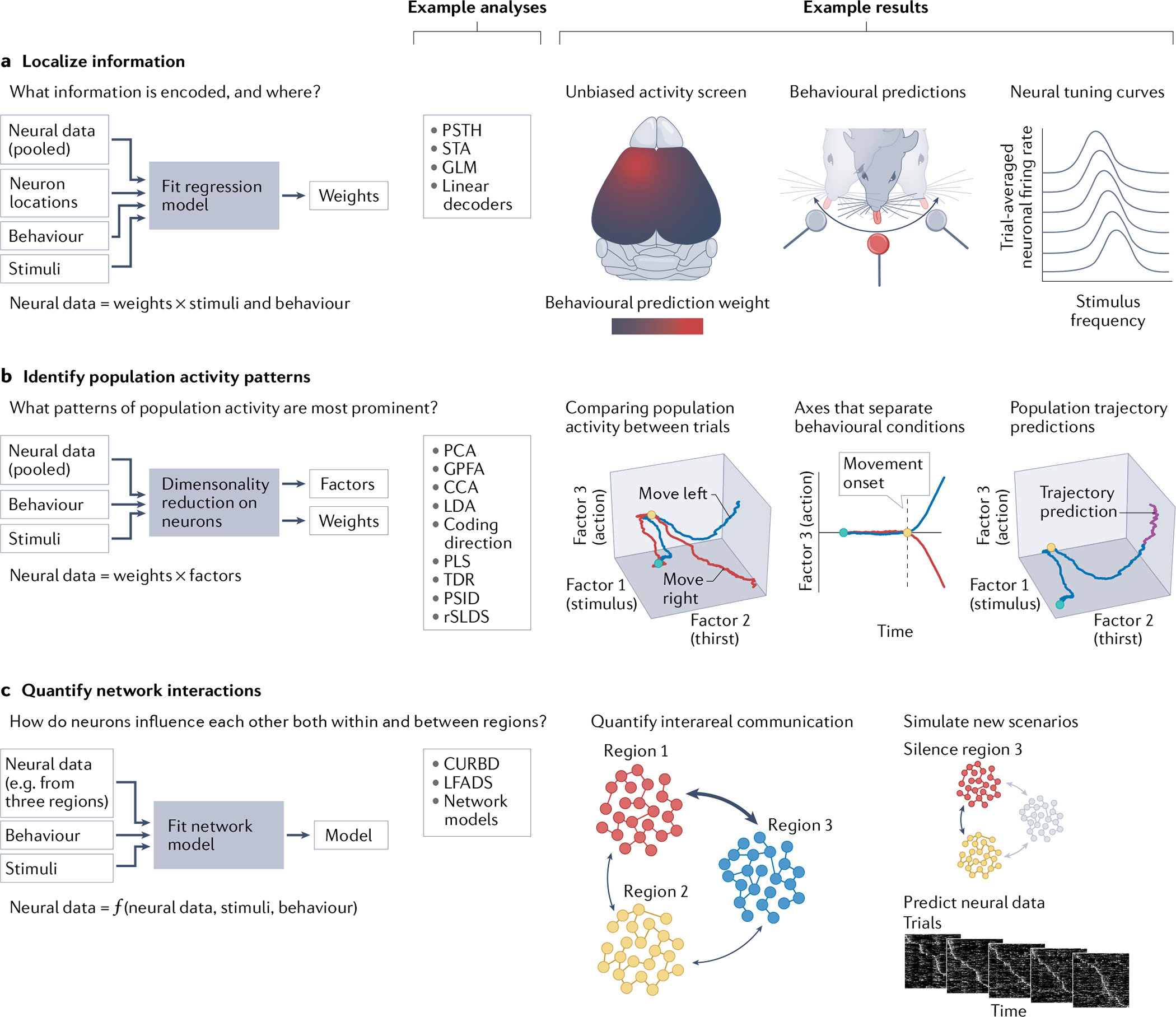
Fig. 2 |. Approaches for analysing multiregion recording data.

There are many approaches for analysing and interpreting multiregion neural data, each of which can address different types of questions. a | What information is being represented by neurons in a dataset? Questions of this nature can be studied using regression models that try to model neural data as a weighted sum of other variables, including information about animal behaviour, experimental stimuli, information about neuronal identity and position, and signals from other neurons. In the unbiased activity screen example (left), the weights obtained from a model might represent the brain areas that are most useful for predicting information about an animal’s behaviour during a task. In other cases (middle), the product of another set of regression weights and neural data may be used to make behavioural predictions (for example, to predict which waterspout the animal might lick to obtain a reward) or compute a neural tuning curve to show the average response of a neuron to a stimulus (right). The algorithm used to compute these weights is often some form of linear regression, such as a generalized linear model (GLM), and may rely on spike-triggered averaging (STA) to reveal the stimulus that a neuron maximally responds to or may rely on computing a trial-averaged response (often called a ‘peristimulus time histogram’ (PSTH)) to reveal the neural response to a specific stimulus. b | What is the regularity and prominence of different patterns of neural population activity? To study this question, dimensionality reduction techniques can be used to compress the activity of hundreds of neurons into a few prominent factors that can then be used to represent the joint activity of a neural population as a low-dimensional trajectory. These algorithms typically attempt to approximate a data matrix of neurons over time (N × T) as the product of a matrix of neuron weights over factors (N × D) and a matrix of factors over time (D × T), where the number of factors (D) is typically set to be some number less than N (often 2–5). This can be accomplished (in use of many algorithms) with different constraints on the features that must be present in the weights and factors (which are sometimes formulated in slightly different ways and may also incorporate information about behaviour, stimuli and how neural signals evolve over time). These methods, which are described in the main text, include principal component analysis (PCA), Gaussian process factor analysis (GPFA), canonical correlation analysis (CCA), linear discriminant analysis (LDA), coding direction analyses, partial least squares regression (PLS), targeted dimensionality reduction (TDR), preferential subspace identification (PSID) and recurrent switching linear dynamical systems (rSLDS). Projecting the neural data into a low-dimensional space defined by factors can be used to construct neural trajectories that can be visualized, quantified and used to compare the joint activity of a neural population across different trials and behavioural conditions (the green dot represents trial onset, the yellow dot represents movement onset and the red and blue lines represent schematic trial-averaged population activity as a mouse prepares to move right or left, respectively; left panel). Specific factors may be constructed to maximally separate population activity trajectories during different behavioural conditions (middle; format matches left panel). Many of these models can also be used to predict how a neural population trajectory might evolve in the future — in the absence of additional neural data (rightmost panel; general form of trajectory matches left panel). c | How do neurons interact with each other both within and between different brain areas? This can be studied by using algorithms such as latent factor analysis via dynamical systems (LFADS) and current-based decomposition (CURBD) to fit network models to datasets consisting of multiregion neural data, information about animal behaviour and sensory stimuli. The fitted network models can then be used to simulate how neural data might be generated by novel sets of stimuli or to generate unique behavioural outputs. Unlike with a real neural dataset, no element of these models is unobservable. Therefore, direct analysis of these models as a surrogate for the neural data of interest can be used, for example, to quantify the direction and strength of interareal communication between distinct brain regions (left). Communication strengths are indicated by the widths of the arrows between the areas. Use of these models also permits simulation of new experimental scenarios (for example, the behavioural and network-wide effects of silencing a set of neurons; right).