Extended Data Figure 8. Phase diagram simulations.

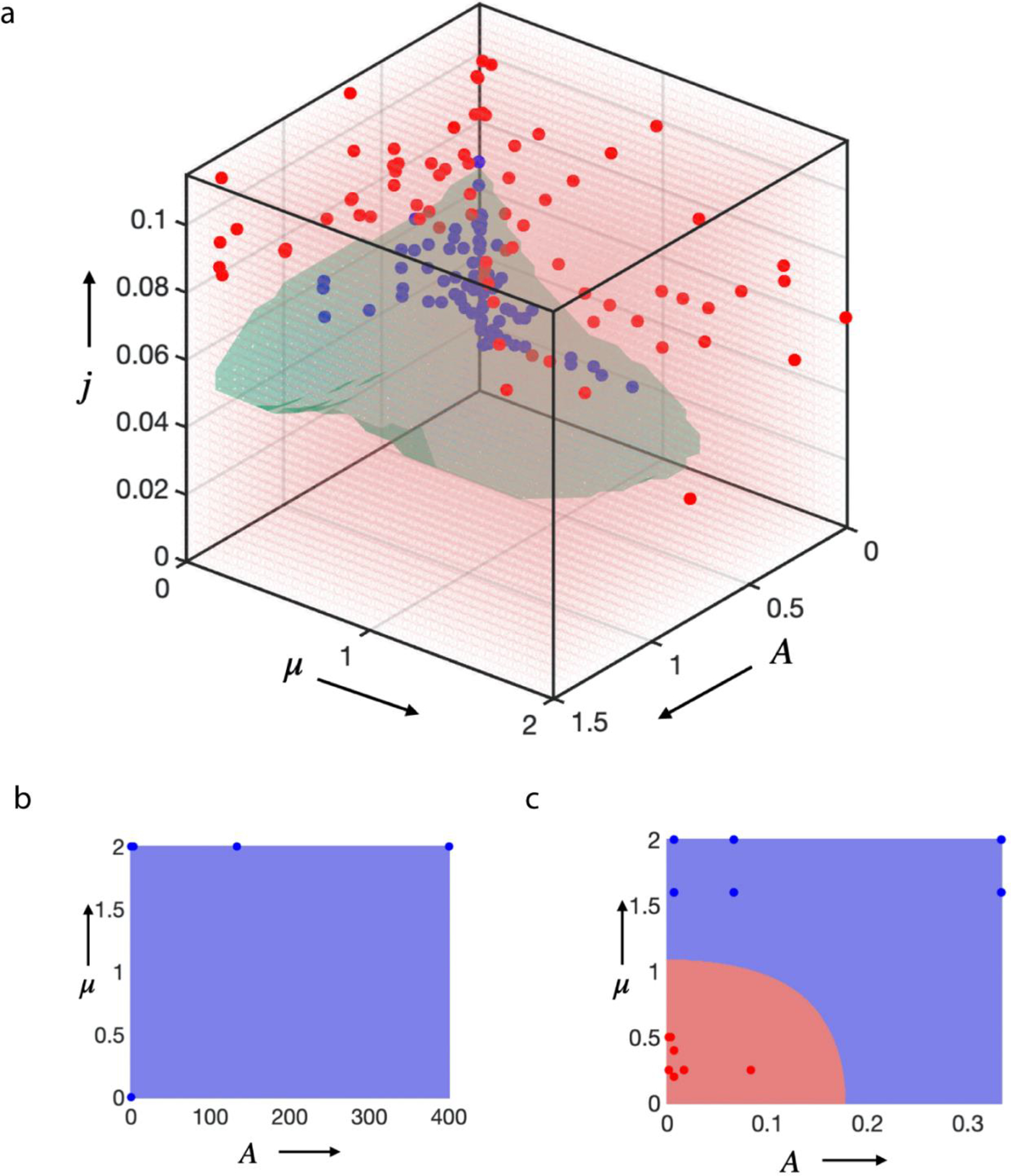
a, 3D phase diagram including the results of multiple simulation runs utilized to determine the phase boundaries. Each dot represents the final result of a single simulation run under specific condition, and they are color coded (blue= stable tissue growth; red=unstable tissue growth). b, A two-dimensional phase diagram for low motility case as a consequence of slow addition of cells, always leading to a stable spheroid (all blue). c, Two-dimensional phase diagram for the controlled cell-flux driven case where the addition of cells is fast. This leads to an inverted behavior, the growth of tissue in elastic matrix (close to origin) is branched (red) and in viscoelastic matrix (away from origin) is a stable (blue). In b and c, the red and blue dots against represent data points extracted from individual simulations. When the scaled proliferation pressure $j=\frac{{\tau }_{\mathrm{g}}}{{\tau }_{\mathrm{t}}}\ll 1$, the tissue grows as a stable spheroid (Fig. 3i,j and Supplementary Fig. 8, 9). Additionally, when the scaled matrix relaxation time $A=\frac{{\tau }_{\mathrm{a}}}{{\tau }_{\mathrm{m}}}\ll 1$, the tissue remains spheroidal and is morphologically stable as long as the scaled proliferation pressure $j=\frac{{\tau }_{\mathrm{g}}}{{\tau }_{\mathrm{t}}}~O(1)$ (top panel of Fig.1d, Fig.3b and Fig.4b). When the scaled matrix relaxation time $A=\frac{{\tau }_{\mathrm{a}}}{{\tau }_{\mathrm{m}}}\gg 1$: if the scaled proliferation pressure $j=\frac{{\tau }_{\mathrm{g}}}{{\tau }_{\mathrm{t}}}\ll 1$, the tissue grows as a stable spheroid (bottom right of Fig. 3i and bottom panel of Supplementary Fig. 8b); if the scaled proliferation pressure $j=\frac{{\tau }_{\mathrm{g}}}{{\tau }_{\mathrm{t}}}~O(1)$, the growth is unstable and the tissue breaks symmetry and develops fingers (bottom panel of Fig.1d and bottom panel of Fig. 3b and 4b); if the scaled proliferation pressure $j=\frac{{\tau }_{\mathrm{g}}}{{\tau }_{\mathrm{t}}}\gg 1$, the morphological stability of the tissue depends on $\mu =\frac{{\mu }_{\mathrm{t}}}{{\mu }_{\mathrm{m}}}$ (see Extended Data Fig 7d,e and 8c); for $\mu =\frac{{\mu }_{\mathrm{t}}}{{\mu }_{\mathrm{m}}}\ll 1$, the tissue remains spheroidal (Extended Data Fig.7d,e, 8c); for $\mu =\frac{{\mu }_{\mathrm{t}}}{{\mu }_{\mathrm{m}}}\gg 1$, growth is unstable and the tissue breaks symmetry and develops fingers (Extended Data Fig.7d,e, 8c).viscoelastic limit are $\left(A=\frac{{\tau }_{\mathrm{a}}}{{\tau }_{\mathrm{m}}}=0.017,\mu =\frac{{\mu }_{\mathrm{t}}}{{\mu }_{\mathrm{m}}}=0.002,j=\frac{{\tau }_{\mathrm{g}}}{{\tau }_{\mathrm{t}}}=0.05\right)$ and $\left(A=\frac{{\tau }_{\mathrm{a}}}{{\tau }_{\mathrm{m}}}=133,\mu =\frac{{\mu }_{\mathrm{t}}}{{\mu }_{\mathrm{m}}}=\right.\left.2,j=\frac{{\tau }_{\mathrm{g}}}{{\tau }_{\mathrm{t}}}=0.16\right)$, respectively.