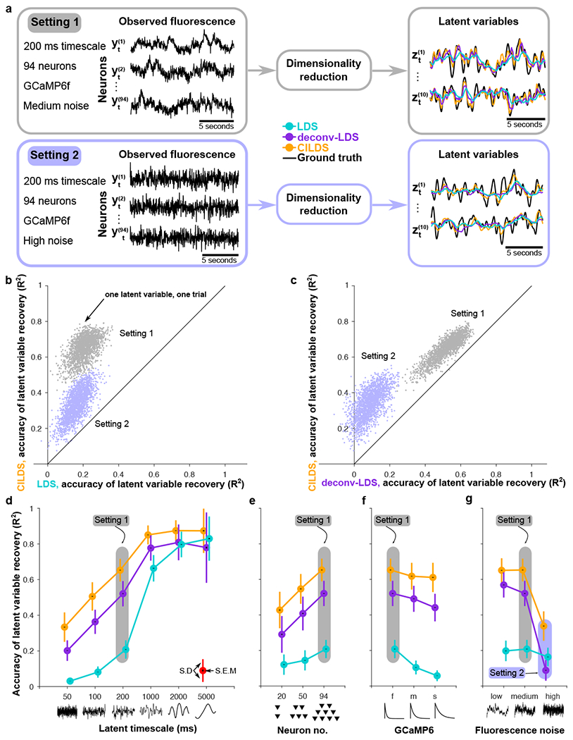
Figure 3: Accuracy of latent variable recovery in simulation.

(a) Example simulated fluorescence traces (left panels) and estimated latent variables (right panels) for two combinations of experimental variables. Setting 1 corresponds to a latent timescale of 200ms, 94 neurons, calcium decay corresponding to GCaMP6f, and medium fluorescence noise (see Methods). Setting 2 is the same as Setting 1, but with high fluorescence noise. Each of the three dimensionality reduction approaches introduced in Fig. 2 (LDS, cyan; deconv-LDS, purple; CILDS, orange) is applied to the simulated fluorescence traces. The latent variables extracted by each method are then compared to the ground truth latent variables (black). (b-c) Accuracy of latent variables estimated by CILDS versus that of (b) LDS and (c) deconv-LDS. Accuracy is measured by the R² between each of the estimated and ground truth latent variables. Each point represents one latent variable on one trial, with a total of 2000 points for each setting, comprising 200 trials and 10 latent variables per trial. (d-g) Mean accuracy of latent variable recovery, as the (d) latent timescale, (e) number of neurons, (f) GCaMP6 indicator decay time constant, and (g) fluorescence noise level was varied. In each panel (d-g), one of the experimental variables was varied, while the other three variables were held constant at the Setting 1 values. The common point across the four panels is Setting 1 (shaded gray). Setting 2 (shaded purple) only appears in panel (g) because panels (d)-(f) correspond to medium rather than high fluorescence noise. The R² for other combinations of experimental variables are shown in Supplementary Fig. 1. Colored error bars indicate standard deviation, and black error bars indicate standard error across n = 2000 latent variables (see Methods). The points are horizontally offset for visual clarity.