Figure 2:

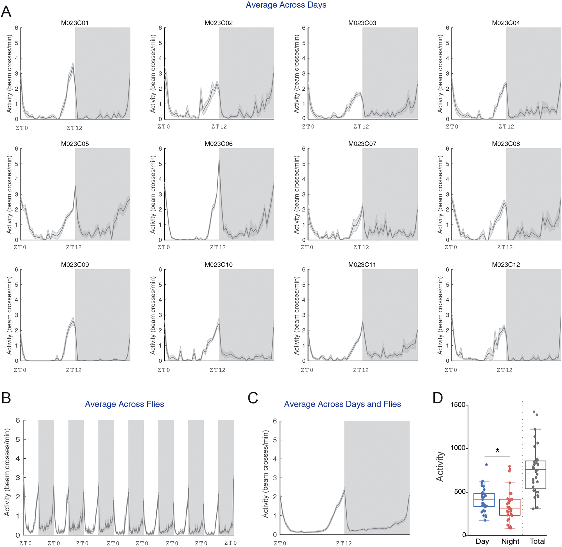
“Averaged Activity Analysis” outputs from PHASE summarizing activity across flies and environmental cycles. Here, example activity time-courses are displayed for male Canton-S (CS) flies recorded under LD12:12 cycles at a constant 25 °C. (A) Averaged activity output from PHASE when time-series are averaged across days for 12 individual flies (see panel A–iii in Fig. 1). (B) Output from PHASE when time-series are averaged across all 32 flies (see panel A–iii in Fig. 1). (C) Output from PHASE when time-series are averaged across both days and flies (see panel A–iii in Fig. 1). Gray shaded regions in panels (A) through (C) indicate the scotophase (i.e., darkness) of the light/dark cycle. When these analyses are executed, corresponding spreadsheets are generated (see user manual for details), which can be used to visualize and perform statistical tests on activity parameters. One such example is shown in (D), wherein total day-time and night-time activity in CS flies is compared. As described previously, day-time activity is significantly higher than night-time activity as judged by a Wilcoxon’s matched pairs test implemented in R (V = 395; p = 0.013; also indicated on the plot using an asterisk). Also shown, for relative comparison, is the total activity counts across one full cycle (not included in any statistical comparisons). Note that such plots can be visualized as normalized time-series using the “Normalized Activity Analysis” output button (Fig. 1A–v).