Figure 6:

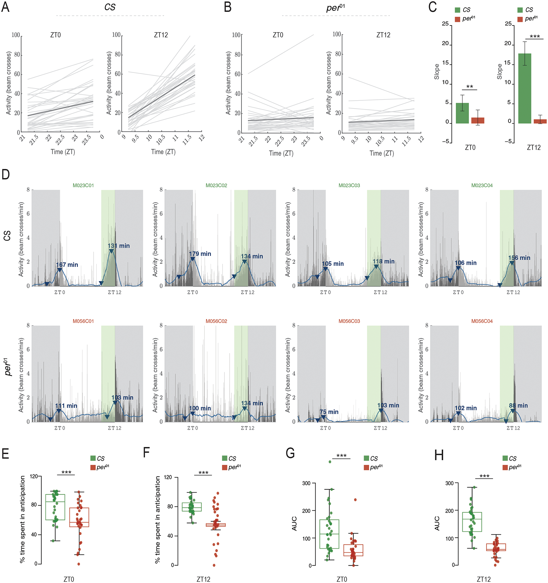
“Anticipation or Latency” outputs from PHASE. Plots indicating slopes of activity levels in user-defined windows for individual male Canton-S (CS) (A) and per⁰¹ (B). Light gray lines represent least squares linear regressions for individual flies, and the dark gray line represents the averaged regression across all flies. (C) The slope values represented in panels (A) and (B) are exported within a PHASE-generated spreadsheet and are used to making comparisons between genotypes or treatments. A population with no anticipation would be expected to show a slope of zero. We performed single-sample t-tests to determine if the mean slope for each genotype was different from zero. CS flies have slope values that are significantly greater than zero in both the morning (left; t₃₁ = 5.2057; p = 1.191e-05) and evening (right; t₃₁ = 12.051; p = 3.118e-13) windows. On the other hand, per⁰¹ flies did not have significant anticipation in the morning (left; t₃₁ = 1.564; p = 0.128) or evening (right; t₃₁ = 1.928; p = 0.063) window. The error bars on these plots are 95% CI based on the reported t-tests. Therefore, any mean with error bars that cross the zero-mark is not different from zero. We also performed Welch’s t-tests to compare anticipation values between CS and per⁰¹ flies in both windows. We found that anticipation in the morning (left; t_61.87 = 2.686; p = 0.009) and evening (right; t_39.04 = 10.669; p = 3.912e-13) windows is significantly greater in CS flies as compared to per⁰¹ mutants. (D) Representative activity profiles (channels 1 through 4) of Canton-S (CS; top) and per⁰¹ (bottom) flies under LD12:12. The thin vertical bars represent the activity of the fly in 1-min bins averaged over all days chosen by the user. The blue line is the smoothed waveform after applying a Savitzky-Golay filter (see text for details). Dark gray shaded region is the scotophase of the light/dark cycle. The green shaded region in the plot (clearly visible before ZT12) is the user-defined window in which anticipation/latency is computed. This green shaded region is not an output of PHASE and has been shown here only for illustration. The blue arrowheads show the minimum and maximum value of activity on the smoothed waveform in the user-defined window. Note that the arrowhead is not displayed for smoothed data points that are negative. The arrowhead marking the maximum value is annotated with the duration of anticipation or latency (in minutes; in other words, duration between the minimum and maximum value). (E-F) Percentage of time spent in anticipation is significantly higher in CS than per⁰¹ flies in both the morning (E; ₁χ² = 13.052; p = 0.0003) and evening (F; ₁χ² = 40.713; p = 1.763e-10) windows. Similarly, areas under the curve (AUC) were also significantly higher in CS than per⁰¹ flies in morning (G; ₁χ² = 19.043; p = 1.278e-5) and evening (H; ₁χ² = 37.324; p = 1e-09) windows. All inferences in panels (B) through (E) were made using Kruskal-Wallis tests implemented in R. For all panels: * < 0.05, ** < 0.01, *** < 0.001, and NS (Not Significant). Note that a similar approach can be used on sleep data to summarize increases in sleep following environmental transitions as a means of quantifying the latency of sleep (see manual).