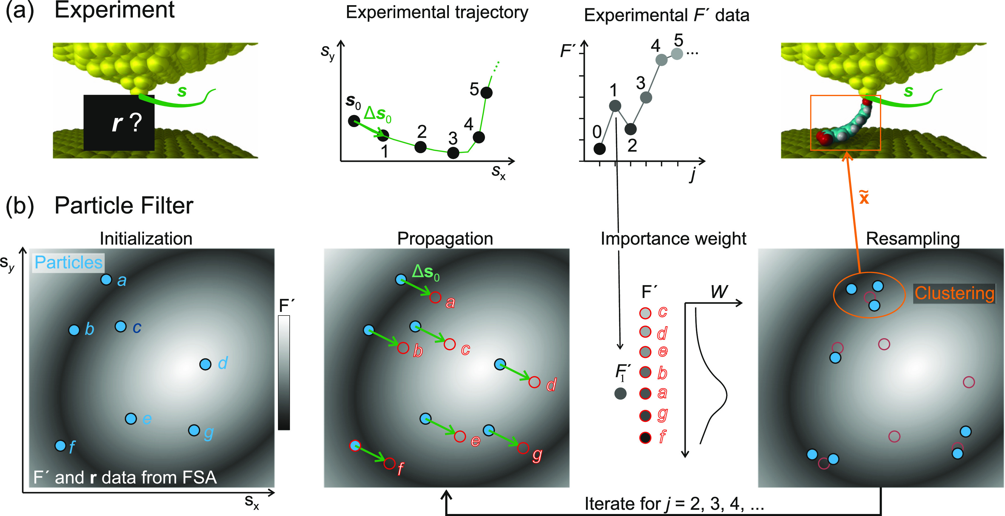
Figure 10.

Operation principle of the particle filter. (a) Experiment. Starting from an unknown molecule configuration r₀, the tip is moved along a trajectory s_j–1, j = 1, ···, 5 in the x,y plane (green), and force gradients F′ (s_j–1) are recorded. (b) Particle filter. Initialization. Particles (G = 7) are dispersed in at random tip–molecule configurations x_l, l = 1, ···, 7 (blue). The gray background symbolizes the observation model F′ = U(x) stored in the FSA. (1) Propagation. All particles are displaced according to the experimental tip displacement step Δs₀ and the state transition model as x_l,1 = S(x_l,0, Δs₀). Synthetic noise in the displacement is omitted here. Each particle l has a distinct F_l^′ (background greyscale). (2) Importance weight. According to the agreement between their F_l value and the experimental F′, the particles receive individual importance weights W_l (eq 9). (3) Resampling. All particles are randomly relocated to the proximity of previous particle locations (faint red), favoring the original locations of particles with high W_l (here: particles a, b, g, and f). Exploration places a fraction ϵ of the particles in completely random locations (not shown). (4) Clustering. Regions with high particle density are identified because they represent the PF’s best estimates of the actual molecular configuration r₁, which is the property of interest. The PF will iterate through steps (1)–(3) for j = 2, 3, ···, converging the particle locations further onto good configuration estimates for x_j. Step (4) is only required when an ad hoc conformation estimate x̃ is requested.