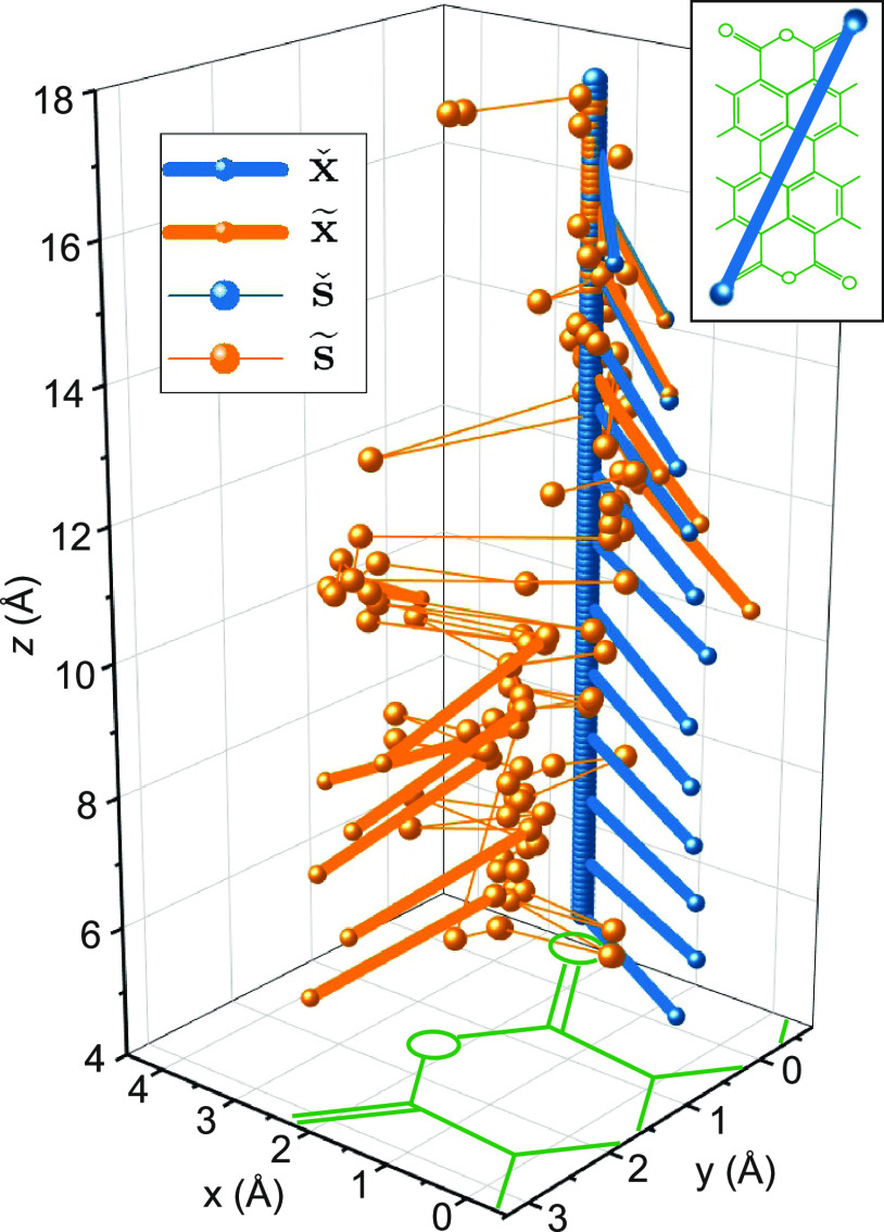
Figure 12.
Ad hoc and consistent trajectories. Example of the x̃j and x̌j configuration estimates in a PF run on a synthetic data set that starts at low sz values. Large spheres mark tip positions, thin lines connect subsequent s̃j points, and thick lines and small spheres visualize the azimuthal orientation of the molecule (see inset) for selected j values. The molecule (green) at the bottom of the main panel is drawn to scale.

