TABLE 3.

Comparative table to show similarities and differences between the methods of assessment of the strength of top‐down and bottom‐up effects using community matrices (left section) and using contribution analysis of birth rate (right section).

Step	Interaction strength in a community matrix		Interaction strength by means of contribution analysis of birth rate
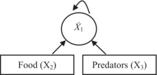
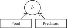
1	A graphical representation of the effect of food (bottom‐up) and predators (top‐down) on
	the population growth rate (Ẋ 1) of a target species		the per capita birth rate (b) of a target species
1a	NA		A graphical representation of the effect of food and size‐selective predators on birth rate, mediated by fecundity (F) and proportion of adults (A), respectively
2	A general model for
	population growth rate		per capita birth rate
	Ẋ 1 = f(X 1, X 2, X 3)		b = g(F, A, V)
3	Decomposition of a change in Ẋ 1 or b into components, each due to a change in the variable involved
	${\dot{X}}_1=\frac{\partial f}{\partial X_1}\mathrm{\Delta }{X}_1+\frac{\partial f}{\partial X_2}\mathrm{\Delta }{X}_2+\frac{\partial f}{\partial X_3}\mathrm{\Delta }{X}_3$		$\mathrm{\Delta }b=\frac{\partial g}{\partial F}\mathrm{\Delta }F+\frac{\partial g}{\partial A}\mathrm{\Delta }A+\frac{\partial g}{\partial V}\mathrm{\Delta }V$
4	A working model for
	population growth rate		per capita birth rate in zooplankton
	${\dot{X}}_1=X_1\left(r_1+\sum _i{a}_{1i}{X}_i\right)i=1,2,3$		b = V ln(1 + FA)
5	Interaction strength measured in terms of
	partial derivatives		partial derivative ∙ Δ(variable) = contribution
	Equation	Type of effect	Equation	Type of effect
	$S_{11}=\frac{\partial f}{\partial X_1}=r_1+2a_{11}{X}_1+\sum _i{a}_{1i}{X}_{i}i=2,3$	Self‐effect (not of interest here)	$\mathrm{Con}F=\frac{\partial g}{\partial F}\mathrm{\Delta }F=\frac{\mathit{VA}}{1+\mathit{FA}}\mathrm{\Delta }F$	Bottom‐up
	$S_{12}=\frac{\partial f}{\partial X_2}=a_{12}{X}_1$	Bottom‐up	$\mathrm{Con}A=\frac{\partial g}{\partial A}\mathrm{\Delta }A=\frac{\mathit{VF}}{1+\mathit{FA}}\mathrm{\Delta }A$	Top‐down
	$S_{13}=\frac{\partial f}{\partial X_3}=a_{13}{X}_1$	Top‐down	$\mathrm{Con}V=\frac{\partial g}{\partial V}\mathrm{\Delta }V=\mathrm{\Delta }V\cdot \text{In}\left(1+\mathit{FA}\right)$	Temperature effect (not of interest here)

Note: The methods are divided into five (community matrices) or six (contribution analysis) steps, as indicated. The main similarity between the methods is that both employ partial derivatives to measure interaction strengths, and the main difference is that contribution analysis, after Caswell (1989), additionally accounts for actual changes in the variables considered so that the strength of the effect is expressed as the partial derivative with respect to a given variable times the actual shift in that variable (Step 5). An additional difference is that contribution analysis of birth rate involves population characteristics (fecundity and proportion of adults) that are intermediate between the environmental factors (food and predation, respectively) and the population's response (Step 1a; this step is not available, NA, in the community matrices method). Community matrices section. X ₁, X ₂, and X ₃ are the abundances of a target species, food, and predators, respectively. Arrows indicate the effect, including a self‐effect (Step 1). In the left‐hand side of the expression for decomposition (Step 3), there is Ẋ ₁ rather than ΔẊ ₁ because the expansion is performed around the equilibrium point at which Ẋ ₁ = 0. The model shown at Step 4 is a generalized Lotka–Volterra model (Yodzis, 1989) commonly used in the context of community matrices (Novak et al., 2016). Contribution analysis of birth rate section. Arrows indicate the effect (Steps 1 and 1a). Predators are assumed to be size‐selective, as is often the case in zooplankton, hence the effect of predators on the proportion of adults A and through A on per capita birth rate b (Step 1a). The model shown at Step 4 and used in this study and elsewhere (Polishchuk, 1995; Polishchuk et al., 2013) is the Edmondson–Paloheimo model of birth rate in zooplankton (Edmondson, 1968; Paloheimo, 1974). Along with fecundity and proportion of adults, the model includes the egg development rate V, which is the reciprocal of the egg development time. The latter is known to largely depend on temperature; its effect on birth rate, and hence the effect of temperature, is not considered here. More information is given in the body of the table.