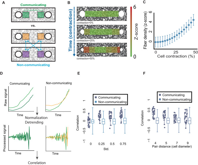
Fig. 2. Using temporal correlations of ECM remodeling fluctuations to distinguish between communicating and non-communicating simulated cell pairs.

A Schematic sketch of comparing ECM remodeling fluctuations of communicating versus non-communicating cell pairs. The correlation between quantification windows of communicating pairs (upper in green) is evaluated in relation to the correlation between two cells from two different communicating pairs (lower in orange and purple). B, C Quantitative visualization and quantification of the dynamics of simulated cell-ECM-cell communication. B Representative simulation visualization at the onset (top), 25% cell contraction (middle), and 50% cell contraction (bottom). C Quantifying fiber densification as a function of simulated contraction steps in between cell pairs. N = 20 cell pairs. Color code (B) and y-axis (C) encode the ECM density in z-score, the number of standard deviations above background levels. The variability in fiber density is a consequence of the randomness in the network architecture. The pair distance between simulated cell centers was set to 7 cell diameters. D Correlation-based pipeline to measure cell-ECM-cell communication in simulations. Raw time series refers to measurement of ECM density in the quantification window (top), normalization with respect to the mean background fiber density at regions that were not influenced by the cells and detrending by second temporal derivative lead to a fluctuating signal (bottom) that is correlated to distinguish between pairs of communicating versus non-communicating cells (left versus right). E Distinguishing between communicating and non-communicating simulated cell pairs correlations of the fluctuations of the second derivative of fiber density with different levels of contraction heterogeneity. Each data point records the correlation between a simulated communicating cell pair, each box plot record the corresponding distribution of correlations between (the many) pairs of non-communicating cells. Mean contraction of 1% and standard deviation (heterogeneity) of 0%, 0.25%, 0.5%, and 0.75%. Three statistical tests are performed according to the following order. (1) Wilcoxon sum-rank testing the null hypothesis that the two correlation distributions of communicating and non-communicating cell pairs are originating from the same distribution. Wilcoxon sign-rank testing the null hypothesis that the correlation distributions of (2) communicating or (3) non-communicating are distributed around a mean 0. Std. = 0%: N = 20, p-values: (1) not significant, (2) not significant, and (3) not significant. Std. = 0.25%: N = 19, p-values: (1) < 0.0001, (2) < 0.001, and (3) not significant. Std. = 0.5%: N = 19, p-values: (1) <0.0001, (2) <0.001, (3) not significant. Std. = 0.75%: N = 20, p-values: (1) <0.0001, (2) <0.001, (3) not significant. F Correlation of communicating versus non-communicating cell pairs using the second derivative of fiber density dynamics as a function of the pair distance. Pair distance: 4 (N = 20 pairs, p-value < 0.0001), 5 (N = 19 pairs, p-value < 0.0001), 7 (N = 19 pairs, p-value < 0.01), and 9 (N = 19 pairs, p-value < 0.01). Data points for non-communicating cell pairs were not displayed in panels E, F because there are too many of them, while the number of data points for communicating cells is much smaller and thus can be plotted.