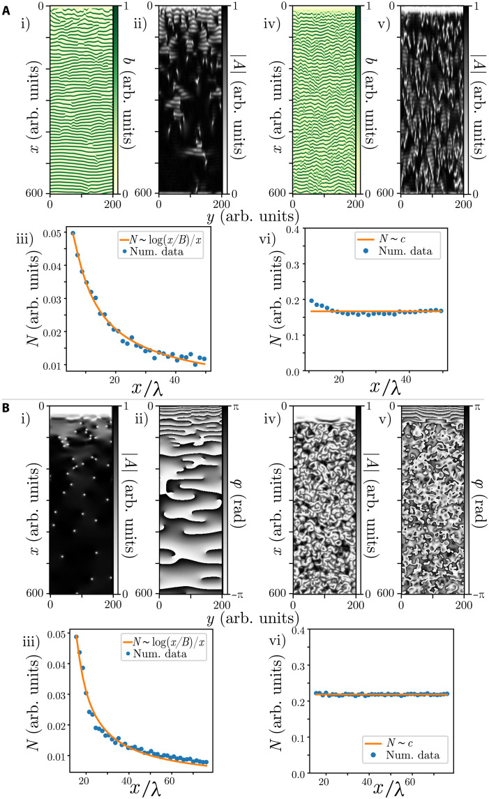
Fig. 5. Transition from nonturbulent to turbulent regime.

(A) Numerical simulations of the weak gradient vegetation model Eq. 2. The real field, the amplitude of the banded pattern, and the defect number distribution. Parameters are η = −0.04, κ = 0.3, p = 0.05, γ = 1.9, for (i) and (ii) α = 1.0, for (iv) and (v) α = 2.0. (iii) and (vi) show the number of dislocations N(x). (B) Numerical simulations of the complex Ginzburg-Landau Eq. 9. Parameters μ(x) = 1 − e^−x/10, ν(x) = 10e^−x/10, $\tilde{\mathrm{\alpha }}=1.0$, for (i) and (ii) β = 0.1, for (iv) and (v) β = 3.0. (iii) and (vi) show the number of dislocations. Fit parameters in λ units are (A, iii) x₀ = 2.7, B = 0.9, and A = 0.1 (R² = 0.99); (B, iii) x₀ = 13, B = 0.7, and A = 0.1 (R² = 0.98). (A, vi) c = 0.16; (B, vi) c = 0.21