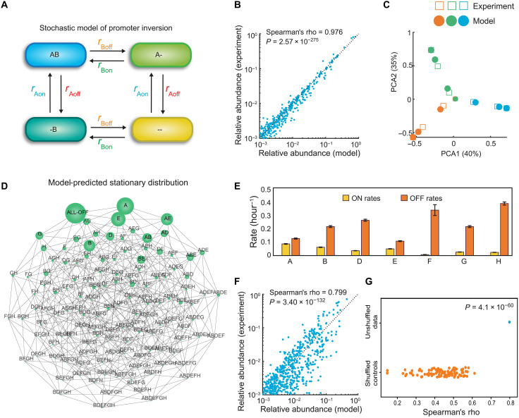
Fig. 4. A stochastic dynamic model of promoter inversions demonstrates that promoter inversion rates shape the trajectory of population diversification.

(A) Schematic (only two promoters) of the stochastic dynamic computational model for capturing temporal changes in single-cell promoter states. In the simplified representation, the cell transitions between four different states by inverting promoters ON and OFF with different kinetic rate parameters. A and B represent different operon promoters in the ON state, and “-” represents the promoter in the OFF state. In the model, there are 7 promoters, 14 kinetic parameters, and 128 different states. (B) Scatter plot of promoter-state relative abundance of the 128 possible promoter combination states predicted by model versus experimentally measured for each time point of the aTc-inducible experiment. Spearman’s rho represents the Spearman correlation coefficient. (C) Model predictions and experimental data visualized using PCA. (D) Undirected network graph of the model’s prediction of the single steady-state promoter l composition (stationary distribution) that all populations eventually converge to. Subpopulations are connected by an edge if their HD is equal to one. Node size represents relative abundance of the subpopulation. (E) Inferred kinetic parameters for promoter inversions derived from the model fitted to the aTc-inducible time-series data. Error bars represent 1 SD of the Markov chain Monte Carlo parameter distribution. Posterior parameter distributions are shown in fig. S7. (F) Scatter plot of promoter-state relative abundance of the 128 possible promoter combination states predicted by model versus experimentally measured for each time point for the 14-day wild-type experiment. (G) Categorial scatter plot of the Spearman’s correlation of a model fit to the label shuffled controls versus wild-type time-series data.