FIG. 10.

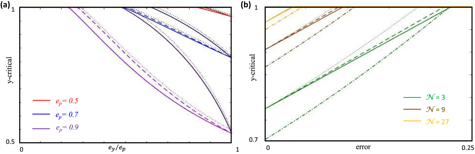
Dependence of y-critical on various parameters for nonzero errors. (a) The red, blue, and purple curves track y-critical as a function of e_y/e_p for e_p = 0.5, 0.7, and 0.9, respectively. The dotted, dashed and bold curves represent the lower bound, leading-order and upper bound y-critical curves for a fixed error, ε = 0.1W. The darker shade correspond to the most nonlinear case when $e_{s\ast }/\sqrt{e_p^2-e_y^2}=1$, while the lighter shade correspond to e_s∗ = 0. These latter curves are also the ones that one obtains in a linear theory. Clearly, the difference between the linear and nonlinear theory increases as e_p increases. In all these cases y-critical decreases with increase of e_p, and for a given e_p, as e_y/e_p increases. Also, as e_s∗ increases and the semiconstrained dimensions become more important, it becomes harder to constrain the synapse sign, and therefore y-critical increases. (b) The green, brown, and orange curves again track y-critical, but this time as a function of ε, for networks with 𝒩 = 3,9, and 27 input neurons, respectively. The dotted, dashed and bold curves plot the lower bound, leading-order and upper bound on y-critical for typical values of e_p, e_y, and e_s∗ that one expects in these networks (B1). We see that these curves come closer together as the network size increases. The dot-dashed curves correspond to the linear theory (e_s∗ = 0), which remains clearly separated from the nonlinear curves. In each of these networks, 𝒫/𝒩 = 2/3 and 𝒞/𝒫 = 1/2.