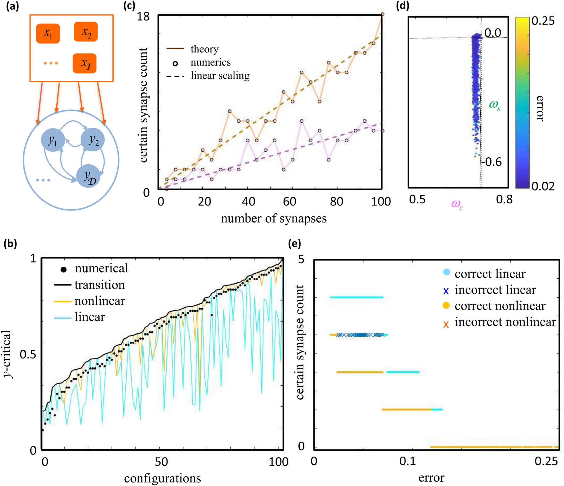
FIG. 8.

The theory accounting for error explains numerical ensembles of feedforward and recurrent networks. (a) Cartoon of a recurrent neural network. We disallow recurrent connectivity of neurons onto themselves throughout this figure. 𝒟 = 1 corresponds to the feedforward case, and W = 1 for all panels. (b) Comparison of numerical and theoretical y-critical values for 102 random configurations of input-output activity (Appendix F). We considered a feedforward network with ℐ = 6, 𝒫 = 5, 𝒞 = 2. For each configuration and postsynaptic activity level y, we used gradient descent learning to numerically find many solutions to the problem with ℇ ≈ 0.1. The black dots correspond to the maximal value of y in our simulations that resulted in an inconsistent sign for the synaptic weight under consideration. The continuous curves show theoretical values for y-critical that upper bound the true y-critical (y_cr,max, black), that neglect topological transitions in the error surface (yellow), or that neglect the threshold nonlinearity (cyan). Only the black curve successfully upper bounded the numerical points. Configurations were sorted by the y_cr,max value predicted by the black curve. (c) The number of certain synapses increased with the total number of synapses in feedforward networks. Purple and brown correspond to 𝒩 = 2𝒫 = 4𝒞 and 𝒩 = 𝒫 = 4𝒞, respectively. The solid lines plot the predicted number of certain synapses. The circles represent the number of correctly predicted synapse signs in the simulations. The dashed brown and purple lines are best-fit linear curves with slopes 0.16(±0.01) and 0.07(±0.01) at 95% confidence level, significantly less than the zero error theoretical estimates of 0.28 and 0.18 (Appendix B). (d), (e) Testing the theory in a recurrent neural network with 𝒩 = 10, ℐ = 7, 𝒟 = 4, 𝒫 = 8, and 𝒞 = 3. Each dot shows a model found with gradient descent learning. (d) x and y axes show two η coordinates predicted to be constrained and semiconstrained, respectively, and the color axis shows the model’s root-mean-square error over neurons, $ℰ/\sqrt{𝒟}$. Although our theory for error surfaces is approximate for recurrent networks, the solution space was well explained by the constrained and semiconstrained dimensions. Note that the numerical solutions tend to have constrained coordinates smaller than the theoretical value (vertical line) because the learning procedure is initialized with small weights and stops at nonzero error. (e) The x axis shows the model’s error, and the y axis shows the number of synapse signs correctly predicted by the nonlinear theory (yellow dots or red crosses) or linear theory (cyan dots or blue crosses). Dots denote models for which every model prediction was accurate, and crosses denote models for which some predictions failed.