

Abstract
During the transportation of oil and gas pipelines, there are many potential factors that can lead to pipeline leakage with serious consequences, making automatic and real-time pipeline leakage detection urgent. In response to the inconvenience of manual detection, constant false alarm rate (CFAR) detection technique in radar target detection theory is introduced for pipeline leakage detection based on acoustic signals. In this paper, an automatic pipeline leakage detection algorithm based on an improved CFAR detector is proposed. The improved CFAR detection is executed after pre-processing the acoustic signals so as to adaptively set the detection threshold to achieve the purpose of automatic detection of pipeline leakage incidents. A simulated leakage test of a real pipeline is used for validation, and the proposed method achieves detection accuracies of 84.6%, 97.7%, and 98% for different leakage diameter settings, i.e., 5 mm, 7 mm, and 10 mm leak hole diameters, respectively, with an overall accuracy of 94.1%, while the false alarm rates are 3.3%, 0.7%, and 0, respectively, as well as an overall of 1.2%. The results of experimental data based on real scenarios demonstrate the effectiveness of the proposed method.
Subject terms: Electrical and electronic engineering, Energy infrastructure
Introduction
Energy transportation is the basis of modern industrialized societies. Connecting energy origins to densely populated consumer markets through energy transportation pipelines1, 2 not only reduces the imbalance between regions, but also reduces emissions in industrialized regions. For example, China’s West-to-East Gas Transmission Project delivers abundant natural gas resources from the west to the resource-poor east to release the contradiction of uneven resource distribution and help improve the fragile environment in the industrialized east3. The first two phases of the West-to-East gas pipeline network currently in operation cover a total distance of nearly 13,000 km. According to the design4, 5, the gas transmission capacity is 12 billion cubic meters in Phase I and 30 billion cubic meters in Phase II. In the face of energy transportation of such scale and length, safe operation is crucial and a major challenge. One of the issues that threatens the safe operation of energy transportation is pipeline leakage. Therefore, pipeline leak detection technology is an important way to ensure the safety of energy pipeline transportation.
Due to the complex terrain and climatic conditions, pipeline laying patterns are diverse6. Complex construction patterns also have more potential factors that lead to leaks. Therefore, leak detection requires an algorithmic model that can detect in real time and dynamically, without the interference of complex environments. Most of the earlier pipeline leak detection relied on manual detection, which greatly reduced the efficiency of detection. Therefore, an automated detection technology is necessary. In addition, it is possible to improve the accuracy of leak detection with the assistance of smart sensors7.
Several studies have been presented to analyze leak signals from oil and gas pipelines. The main focus in these studies was on acoustic sensor signals. Fuchs and Riehle demonstrated the feasibility of using acoustic fields for leak detection, which have been widely used for leak measurements8. Hou and Zhang proposed the use of the negative pressure wave principle for leak signal detection9. Wan10, Gao11 and Mostafapour12 also proposed to connect to two or more sensors to collect data for analysis. The analysis results show that the leakage signal is highly attenuated by the acoustic energy in the pipeline, and the attenuation is particularly pronounced in the high frequency component. Most of these findings are presented in terms of acoustic model characteristics. They clarify many of the main physical properties of the leak signal and the methods for capturing and analyzing it. However, they only emphasized the methods that rely mainly on manual supervision. Very little research has been done on detection algorithm models.
Based on the above analysis, this paper focuses on the study of automatic algorithms used for pipeline leak detection. An algorithmic model capable of automatically detecting pipeline leaks will be proposed. It will replace the previous manual monitoring or fixed-threshold detection methods, whose thresholds can be dynamically adjusted in real time according to the amplitude of the noise level, thus achieving a balance between false alarm probability and detection probability. To achieve this goal, the constant false alarm rate detector13 in radar detection theory is used for the real-time detection of pipeline leakage signals. Constant false alarm rate (CFAR) detector is an adaptive threshold method that detects the target with a constant false alarm probability level, which eliminates the problem of threshold failure due to noise level variations. Its real-time threshold adjustment property makes it an effective method for automatic detection and facilitates real-time implementation with less computation compared to machine learning based methods14–16. To the best of our knowledge, this is the first time that the idea of CFAR detection is applied to pipeline leakage detection.
The rest of the paper is organized as follows. “Pipeline leakage acoustic signal model” models the acoustic signatures of pipeline leaks. Then an automatic leak detection method based on CFAR is presented in “Pipeline leak detection based on constant false alarm rate detector”. Real-world experiment based results are shown and discussed in “Experimental results and discussion”. Finally, “Conclusion” concludes this paper.
Pipeline leakage acoustic signal model
For pipeline leakage events, there are two types of situations that may be encountered: normal operating situation and leakage situation. The acoustic signals for each of the two cases will be modeled as follows.
Signal model in normal operating situation
When no leakage occurs, the pipeline transport is in normal working condition, at this time the acoustic sensor will not receive abnormal signals, and the signal in this case can be modeled as Gaussian white noise as follows:
| 1 |
where t is the time, s is the signal amplitude at time t, is the expectation of the noise signal, and is the variance of the noise signal.
In practical scenarios, the noise acquired by acoustic sensors mainly comes from thermal noise in circuit devices. Meanwhile, there may be some interference terms, such as electromagnetic interference or operating conditions variations of the transport pump. This makes the mean value of the noise may not be zero. That is, the noise signal is superimposed on some constant term. In addition, if the interference term may change with time, the noise signal will also have a trend term. In this case, the signal can be modeled as
| 2 |
where is the trend term which can change with time.
Signal model in leakage situation
In general, the unstable motion of the fluid or gas during a pipeline leak causes the pipeline near the leak point to vibrate, which in turn causes oscillations in the acoustic signal. In this case, the oscillation of the signal can be summarized as follows:
The amplitude of the signal envelope follows an exponential decay.
Most of the amplitude and energy are concentrated in the transient phase of vibration.
The model of acoustic wave propagation in an ideal fluid medium in a pipeline is17, 18
| 3 |
where x is the direction of propagation, is the sound pressure, and c is the speed of sound in air. The expression for the acoustic pressure solution of (3) with respect to plane waves in the pipeline is
| 4 |
where is the sound pressure amplitude, is the angular frequency, and is the wave number, the represent m-order column Bessel function with the argument of , r and are the radial coordinates and the polar angle in the cylindrical coordinate system, respectively. Therefore, the main component of the acoustic signal model is the product of the exponential decay function and the cosine function.
Considering the noise effect, the model can be expressed as
| 5 |
In addition, in the process of pipeline transportation, due to changes in working conditions or the pump’s own parameters. There is also a slow-varying trend term in the acoustic signal. Therefore the final signal model is a combination of acoustic signal, noise and trend term. As shown below.
| 6 |
where is slow change trend term.
Pipeline leak detection based on constant false alarm rate detector
Preprocessing of acoustic signals
As mentioned above, the detecting equipment will encounter the environment of pump condition changes and electromagnetic interference during operation. This causes the signal to have a slow-varying trend term. Also, thermal noise exists in the sensor circuit. These factors can lead to false alarms or missed alarms during the detection process and cause interference in the detection of the signal. Therefore, preprocessing of the acoustic signal is required.
Data outlier elimination
In the process of signal acquisition by the sensor, there may be a moment of data loss due to the instability of the network environment during the transmission process, generating some abnormal data. When the data loss occurs, the abnormal signal usually produces a mutation point. In order to prevent this abnormal signal from being misjudged as a leak incident, special numerical processing of this abnormal signal is required to avoid the impact on the detection results.
Since outliers in a signal are usually characterized by randomness and sparse distribution. Median filtering can be used to process the outliers. The median filtering is realized as follows.
| 7 |
where t denotes the time, is the original signal, is the sorting function, is the median taking operation, and w(n) is a moving window defined as follows,
| 8 |
where N is the window length, and nan represents a non-existent value.
Data de-trending
In the process of media transmission in the pipeline, there may be a trend of slow change in the signal due to the change of working conditions, which makes the detection threshold may also fluctuate, resulting in false alarms or missed detections. Thus the trend of the signal need to be removed before leakage detection. By using the moving window difference, the signal trend can be eliminated. The moving window difference is realized as follows.
| 9 |
where N is the moving window length.
Data denoising
During the collection of acoustic signals, thermal noise in the sensor circuit is also recorded along with the acoustic waves. Therefore, after cleaning the data outliers and removing the trend components, the signal also needs to be processed for noise reduction to further improve the signal-to-noise ratio (SNR) and facilitate subsequent leak incident detection. The noise in the signal can be suppressed by moving mean. The implementation process is as follows.
| 10 |
Introduction of CFAR detector
After performing signal preprocessing, the power signal can be obtained as follows and used as input for a CFAR detector:
| 11 |
The CFAR detector is a technique for detecting a target in noise signals while maintaining a constant probability of false alarms. It has been widely used in radar target detection19. Compared with the detection technique with fixed threshold, whose performance degrades when the signal noise level changes, it can maintain better detection performance when the noise level changes due to the adaptive nature of its detection threshold. Therefore, the CFAR will be used in this paper to detect leakage events in acoustic signals.
In radar target detection, the probability of presence of a target under certain conditions is often unknown, nor is the loss caused by a missed detection. Therefore, the Neyman–Pearson criterion is often used in target detection, i.e., given the probability of false alarm condition to maximize the detection probability. To achieve this goal, two hypotheses are defined as follows,
| 12 |
where hypothesis indicates that there is only Gaussian white noise in the current signal and no target is present. hypothesis indicates the presence of a target in the current signal, and the signal consists of a target plus Gaussian white noise.
When the hypothesis holds, i.e., only noise is present, the probability density function of the received signal is
| 13 |
and when the hypothesis holds, i.e., the target and the noise exist simultaneously, the probability density function of the received signal is
| 14 |
then the determination criterion for target detection is
| 15 |
where, the likelihood ratio threshold is a variable proportional to the detection threshold . Under hypothesis , the probability of false alarm due to noise level exceeding the detecting threshold is expressed as
| 16 |
where represents the event that the target is detected, is determined by the assumption that is a constant as shown in Fig. 1. It can be seen from Fig. 1, the green curve is the probability density function in hypothesis, and the blue curve is the probability density function in hypothesis. Then the false alarm probability is equal to the area of the green curve in the right part of the detection threshold. When the area of this part is constant, i.e., the false alarm probability is constant, the detection threshold can be determined. Then the likelihood ratio threshold can be obtained by the normal inverse cumulative distribution function according to .
Figure 1.

Schematic diagram of the probability distribution of CFAR detection.
In this case, the detection probability can be obtained as
| 17 |
In the specific implementation of CFAR, given a cell under test (CUT), it is necessary to determine the guard region and the training region, and then estimate the noise level based on the value of the training cells, and thus obtain the detection threshold as follows
| 18 |
where q is a scaling factor related to . By choosing a suitable scaling factor, the false alarm probability can be kept as a proper constant. denotes the estimated noise power, For each CUT, the noise power can be obtained by calculating the average value of the training cells as follows.
| 19 |
where M denotes the number of training cells20–22.
It is worthwhile to note that the function of the guard cells is to define a neighborhood around the cell under test (CUT) so that the cells within that neighborhood will not be used for noise level estimation, as shown in Fig. 2. The larger the number of guard cells, the farther the training cells are from the CUT. In practice, the leakage signal is not an ideal impact function but occupies a certain width, in this case, the selection of the guard cells should be at least larger than the width of the leakage signal, otherwise a part of the leakage signal will be used for the noise estimation, thus affecting the setting of the constant false alarm threshold.
Figure 2.

CFAR detection parameters configuration diagram.
The function of the training cells is used for the estimation of the noise level, as shown in Figs. 1 and 2. The noise level is estimated using sample mean, so the accuracy of the noise level estimate depends on the number of training units. Different number of training cells will give noise levels with different estimation accuracy.
The false alarm rate acts as a compromise between the false alarm and detection ability as shown in Fig. 1, i.e., the choice of the threshold determines the false alarm rate setting and the detection probability. If a higher false alarm rate is accepted, then it will also result in a higher detection probability.
The traditional CFAR detection is performed by selecting training cells on the both left and right sides of the CUT23, 24. However, in this work, the pipeline leakage occurs instantaneously. To ensure that the response time for detection is as short as possible, the training cells should not use samples after the moment of the CUT, so the left regions of the CUT are used as the training cells. The schematic diagram of the selection of the training unit is shown in Fig. 2.
Pipeline leakage detection algorithm
Based on the above analysis, the pipeline leakage detection algorithm flow by CFAR is summarized as shown in Fig. 3.
Figure 3.
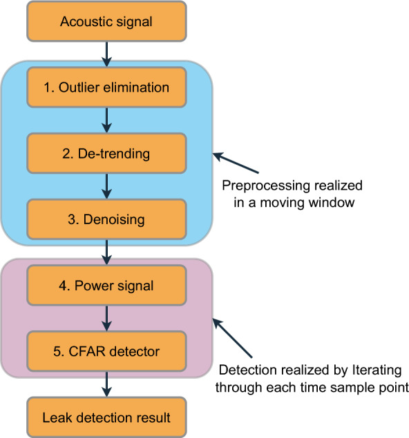
Algorithm flow chart.
In total, the detection algorithm is divided into two main parts: signal preprocessing and leak incident detection. The algorithm modules are described in detail as follows.
Outlier elimination: outliers are usually characterized by randomness and sparsity, so median filtering is used to eliminate them. Here, the time sampling points are processed sequentially using a moving window.
De-trending: detrending: processing in a moving window, the first and last points of the signal intercepted by the window function are differenced to achieve the removal of the trend term.
Denoising: processing using moving window averaging.
Power signal: power signal generation: CFAR detection is based on the power signal, so the power of the acoustic signal needs to be considered to ensure that the negative values in the signal do not affect the detection effect.
CFAR detector: finally, the CFAR detector averaged over the left side cells is used to perform the detection of pipeline leakage signals.
It is worth noting that in the actual implementation of the algorithm, the selection of the number of guard and training cells needs to take into account the duration of the acoustic signal at the time of the leakage incident. The general rule is that the guard cells should be able to effectively cover the length of the acoustic signal in order to ensure that the leakage incident signal is not treated as a noise term for noise level estimation. Meanwhile, due to the presence of the training and guard cells, there will be some detection blind areas in the left boundary part of the signal. However, these detection blind areas have been detected in historical time and thus do not affect the detection capability of the real-time system.
Experimental results and discussion
The design of real-world simulation experiment
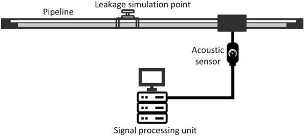
The schematic of the real-world leakage simulation test is shown in Fig. 4. In this experiment, acoustic sensors were installed on the pipeline to collect acoustic signals. An artificial leak point was set up in the middle of the pipeline to simulate a pipeline leak incident. When the valve at the leak point is opened, the transmission medium in the pipeline is released from the leak point, generating a leak acoustic signal that is recorded by the sensors. The data received by the acoustic sensors is converted to a digital signal by an analog-to-digital converter and transmitted to a central computer, which processes the digital signal to determine whether a leak has occurred.
Figure 4.
Schematic diagram of the experimental design.
This real data was collected from a simulated leak test of a pipeline. The data collection time was 2 min, and the sampling period of the sensors was set to 10 ms. The total length of the pipeline was 78.3 km, and the experiment was carried out in the form of a simulation test with a fast-opening and fast-closing valve at 49.8 km from the first station of the pipeline to simulate the leak incident with a leak hole diameter of 5 mm, 7 mm, and 10 mm, respectively. The photographs of the experiment site are shown in Fig. 5.
Figure 5.

Pipeline leakage simulation test site photos. (a) Acoustic sensor installation location; (b) artificially simulated leak point location.
The acoustic signal of a typical pipeline operation is shown in Fig. 6. A digital signal for normal operation and a digital signal for the occurrence of a leakage incident are given, where the vertical coordinate represents the quantized sampling value of the voltage, from which it can be seen that when a leakage occurs, there will be a more distinct change in the signal characteristics.
Figure 6.

Pipeline signals. (a) Normal signal; (b) leak signal.
Experimental results
Signal preprocessing results
For the acoustic signals containing leakage events which occurs at 40.8 s, the results after preprocessing are shown in Fig. 7. It can be seen from the original signal shown in Fig. 7a that it contains more obvious trend term and noise. The trend is caused by the change of working conditions in the pipeline. The noise, on the other hand, originates from the thermal noise of the sensor circuit. After the de-trending process, it can be seen from Fig. 7b that the slow trend of the signal is eliminated, while the characteristics of the leakage signal are retained. After further denoising process, the noise in the signal is suppressed and the leakage signal features are more obvious as shown in Fig. 7c. Finally, the power signal is calculated as shown in Fig. 7d.
Figure 7.

Preprocessing results of leak acoustic signal. (a) Original signal; (b) difference signal; (c) denoised signal; (d) power signal.
Comparing the original signal, it can be seen that the preprocessing eliminates the factors in the signal that are detrimental to the detection of leakage events, making the leakage incident signal more significant and making the subsequent detection process more robust.
Evaluate the impact of different parameter settings of the CFAR detector
The parameters that need to be set during the implementation of the CFAR detector are the number of guard and training cells, and the false alarm rate. The effectiveness of the detector is related to these parameter settings. The relationship between detection results and CFAR parameter settings is given in this section for a reference during practical implementation.
Firstly, the detection effect is evaluated as the number of guard cells increases. The number of guard and training cells is converted into the length of time based on the sampling interval in order to compare with the actual occurrence time. In this case, the training cells and the false alarm rate are fixed as 10 s and respectively. The guard cells are set to 5 s, 10 s, 20 s, and 30 s, respectively for evaluating the leak detection effect. The results are shown in Fig. 8.
Figure 8.

Detection of leak signal in different guard cells setting. (a) 5 s; (b) 10 s; (c) 20 s; (d) 30 s.
As can be seen, when the guard cells are small, such as set to 5 s and 10 , the length of the guard cells cannot cover the whole segment of the leakage signal, which makes the front part of the leakage signal used as the training cells and thus raises the detection threshold, resulting in the back part of the leakage signal cannot be effectively detected as shown in Fig. 8a,b. When the guard cells are set to 20 s and 30 s, the length of the guard cells is already longer than the 17 s length of the leakage signal, so the whole section of the leakage signal can be effectively detected as shown in Fig. 8c,d. In addition, it is worth noting that when the guard cells are set too long, it will increase the length of the detection blind zone as shown in Fig. 8d. Therefore, in this experiment, the guard cell setting of 20 s is appropriate.
Then, the detection effect is evaluated as the number of training cells increases. In this case, the guard cells and the false alarm rate are fixed as 20 s and respectively. The training cells are set to 1 s, 5 s, 10 s, and 20 s, respectively for evaluating the leak detection effect. The results are shown in Fig. 9.
Figure 9.

Detection of leak signal in different training cells setting. (a) 1 s; (b) 5 s; (c) 10 s; (d) 20 s.
It can be seen that when the training cells are small, such as the training cells are set to 1 s, only a small amount of training data is involved in the estimation of the noise level, which makes the estimated value of the noise level fluctuating greatly due to the change of the moving window, thus failing to achieve a good detection effect, and even failing to detect valid signals and making false alarms as shown in Fig. 9a. As the length of the training cells increases, the detection effect gradually improves, and when the training cells are set to 10 s and 20 s, the leakage signal can already be detected correctly Fig. 9c,d. It is worth noting that when the training cells are too large, it increases the amount of training data, making the computation time grow, which in turn affects the real-time performance of the system and increases the difficulty and cost of system implementation. Therefore selecting the appropriate training cells is necessary in practice.
Finally, the detection effect is evaluated as the change of the false alarm rate. In this case, the training and guard cells are fixed as 10 s and 20 s, respectively. The false alarm rate is set to , , , and , respectively for evaluating the leak detection effect. The results are shown in Fig. 10.
Figure 10.

Detection of leak signal in different false alarm rate setting. (a) ; (b) ; (c) ; (d) .
It can be seen that when the false alarm rate is large, it is easy to detect noise as a leakage signal, making the detection results erroneous as shown in Fig. 10a,b. This can be costly in practice in terms of operating costs. As the false alarm rate decreases, the detection threshold is gradually increased so that the leakage signal is detected correctly without false alarms as shown in Fig. 10d. Therefore, in practice, it is necessary to determine the appropriate false alarm.
Multiple experimental results and runtime evaluation
The results of the multiple tests are shown in Table 1. A total of 324 simulated leakage tests are conducted to verify the detection accuracy of the proposed detection method.
Table 1.
Multiple detection results based on simulation test.
| Test index | Leak hole diameter (mm) | Total test number | Number of the detectable | Number of the missed | Number of false alarm | Correct rate (%) | False alarm rate (%) |
|---|---|---|---|---|---|---|---|
| 1 | 5 | 91 | 77 | 11 | 3 | 84.6 | 3.3 |
| 2 | 7 | 133 | 130 | 2 | 1 | 97.7 | 0.7 |
| 3 | 10 | 100 | 98 | 2 | 0 | 98 | 0 |
| Total | – | 324 | 305 | 15 | 4 | 94.1 | 1.2 |
There are a total of 91 leakage tests for the 5 mm diameter, 133 leakage tests for the 7 mm diameter, as well as 100 leakage tests for the 10 mm diameter. In the 5 mm diameter test, 77 leaks are successfully detected, 11 leaks are missed, and 3 false alarms occur. In the 7 mm diameter test, 130 leaks are successfully detected, 2 leaks are missed, and 1 false alarm occurs. In the 10 mm diameter test, 98 leaks are successfully detected, 2 leaks are missed, and there are no false alarms. Correct detection rates of 84.6%, 97.7% and 98% are achieved for the three leak diameter settings, respectively. The overall correct rate is 94.1% in all tests.
From the test results, it can be seen that when the leakage diameter decreases, the correct detection rate decreases and false alarms increase. The reason for this is that the SNR of the acoustic signal decreases when a small diameter is leaked, which reduces the difference between the signal distribution and the noise distribution shown in Fig. 1, thus leading to an increase in the false alarm rate and a decrease in the detection probability. A missed detection sample and a false alarm sample in 5 mm diameter are given in Fig. 11. It can be seen that the SNR is low at this point and the signal of the leakage incident is no longer apparent.
Figure 11.

Anomaly detection samples. (a) Missed detection; (b) false alarm.
The results of the multiple simulation tests demonstrate the effectiveness of the proposed method in real-world scenarios.
We also evaluate the running time of the proposed method. The runtime of the proposed method is tested using data from one leak test. The computer configuration used in this test is as follows.
CPU: Intel i5 8300H
Memory capacity: 8 GB
Operating system: Windows 11
In this configuration, the time to process one test data, i.e. 2 min length of data is 4 s. With a better test platform, such as an embedded platform, the computation time would be reduced to meet the actual real-time detection requirements.
Discussion of multi-leak incident detection
When leaks occur simultaneously at different locations in a pipeline, for a single acoustic sensor, the leak signals generated at different leak locations have different positions in the received signal due to the different arrival times at the sensor. In this case, detection is still possible. In addition, if the distance between different leak locations is far enough to cause the detection signal-to-noise ratio to be too low, it is also possible to consider segmenting the pipeline by distance and installing sensors on different segments to cover the needs of pipeline monitoring over long distances in practice.
Conclusion
In order to overcome the disadvantages of manual detection such as high cost, poor real-time and low accuracy. An automatic pipeline leak detection algorithm based on acoustic signals is proposed by drawing on the CFAR detection technique in radar target detection theory. Based on the real-world experiment data, the detection effect under different CFAR detector parameters is analyzed, and the results show that the proposed method can obtain a better automatic detection effect under the appropriate CFAR detection parameter settings. The results of multiple experiments verify the effectiveness of the proposed method in practical scenarios.
Acknowledgements
This work was supported by the Fundamental Research Funds for the Central Universities 2022RC008.
Author contributions
Y.L. conceived the idea, G.A. and Z.H. proposed the methodology, G.A. and Z.H. verified the method, G.A. and Z.H. analyzed the results. All authors reviewed the manuscript.
Data availability
The datasets used and/or analysed during the current study available from the corresponding author on reasonable request.
Competing interests
The authors declare no competing interests.
Footnotes
Publisher's note
Springer Nature remains neutral with regard to jurisdictional claims in published maps and institutional affiliations.
References
- 1.Ling Z, et al. Omi-measured increasing so 2 emissions due to energy industry expansion and relocation in Northwestern China. Atmos. Chem. Phys. 2017;17:9115–9131. doi: 10.5194/acp-17-9115-2017. [DOI] [Google Scholar]
- 2.Ling Z, et al. Sulfur dioxide pollution and energy justice in Northwestern China embodied in west-east energy transmission of China. Appl. Energy. 2019;238:547–560. doi: 10.1016/j.apenergy.2019.01.123. [DOI] [Google Scholar]
- 3.Wang F, et al. Tracing China’s inter-regional cost transfer of air pollution through domestic supply chains. J. Clean. Prod. 2020;268:121488. doi: 10.1016/j.jclepro.2020.121488. [DOI] [Google Scholar]
- 4.Chen W, Li H, Wu Z. Western China energy development and west to east energy transfer: Application of the western China sustainable energy development model. Energy Policy. 2010;38:7106–7120. doi: 10.1016/j.enpol.2010.07.029. [DOI] [Google Scholar]
- 5.Feng Y, et al. Fracture control of the 2nd west to east gas pipeline in China. Proced. Struct. Integrity. 2019;22:219–228. doi: 10.1016/j.prostr.2020.01.028. [DOI] [Google Scholar]
- 6.Yin P, et al. Influence of aqueous foam on gas-liquid flow development of hilly-terrain wet gas pipeline with surfactant injection. Chem. Eng. Sci. 2023;20:118469. doi: 10.1016/j.ces.2023.118469. [DOI] [Google Scholar]
- 7.Shao Y, Chen C, Lu Z, Zheng Y, Zhang Y. An intelligent leakage detection method for diaphragm wall joints based on fiber Bragg grating sensors and intelligent algorithms. Measurement. 2022;197:111339. doi: 10.1016/j.measurement.2022.111339. [DOI] [Google Scholar]
- 8.Fuchs HV, Riehle RT. years of experience with leak detection by acoustic signal analysis. Appl. Acoust. 1991;33:1–19. doi: 10.1016/0003-682X(91)90062-J. [DOI] [Google Scholar]
- 9.Hou CX, Zhang EH. Applied Mechanics and Materials. Trans Tech Publishing; 2013. Pipeline leak detection based on double sensor negative pressure wave; pp. 1225–1228. [Google Scholar]
- 10.Wan J, Yu Y, Wu Y, Feng R, Yu N. Hierarchical leak detection and localization method in natural gas pipeline monitoring sensor networks. Sensors. 2011;12:189–214. doi: 10.3390/s120100189. [DOI] [PMC free article] [PubMed] [Google Scholar]
- 11.Gao Y, Brennan MJ, Joseph PF, Muggleton JM, Hunaidi O. A model of the correlation function of leak noise in buried plastic pipes. J. Sound Vib. 2004;277:133–148. doi: 10.1016/j.jsv.2003.08.045. [DOI] [Google Scholar]
- 12.Mostafapour A, Davoudi S. Analysis of leakage in high pressure pipe using acoustic emission method. Appl. Acoust. 2013;74:335–342. doi: 10.1016/j.apacoust.2012.07.012. [DOI] [Google Scholar]
- 13.Weinberg GV. Interference control in sliding window detection processes using a Bayesian approach. Digit. Signal Process. 2020;99:102658. doi: 10.1016/j.dsp.2020.102658. [DOI] [Google Scholar]
- 14.Richards MA. Fundamentals of Radar Signal Processing. McGraw-Hill Education; 2014. [Google Scholar]
- 15.Minkler, G. & Minkler, J. Cfar: The principles of automatic radar detection in clutter. NASA STI/Recon Technical Report A 90, 23371 (1990).
- 16.Banjara NK, Sasmal S, Voggu S. Machine learning supported acoustic emission technique for leakage detection in pipelines. Int. J. Press. Vessels Pip. 2020;188:104243. doi: 10.1016/j.ijpvp.2020.104243. [DOI] [Google Scholar]
- 17.Lawrence EK, Coppers AB, Vsanders J, Austin F. Fundamentals of Acoustics. 4. Wiley; 2000. [Google Scholar]
- 18.Fuller C, Fahy FJ. Characteristics of wave propagation and energy distributions in cylindrical elastic shells filled with fluid. J. Sound Vib. 1982;81:501–518. doi: 10.1016/0022-460X(82)90293-0. [DOI] [Google Scholar]
- 19.de Medeiros DDS, da Costa RF, Alves DI, Machado R, Saotome O. Remote Sensing of the Ocean, Sea Ice, Coastal Waters, and Large Water Regions 2022. SPIE; 2022. High-frequency surface wave radar performance analysis for ca-cfar algorithm in Weibull-distributed clutter; p. 1226302. [Google Scholar]
- 20.Himonas SD, Barkat M. Automatic censored cfar detection for nonhomogeneous environments. IEEE Trans. Aerosp. Electron. Syst. 1992;28:286–304. doi: 10.1109/7.135454. [DOI] [Google Scholar]
- 21.Smith ME, Varshney PK. Intelligent cfar processor based on data variability. IEEE Trans. Aerosp. Electron. Syst. 2000;36:837–847. doi: 10.1109/7.869503. [DOI] [Google Scholar]
- 22.García FDA, Rodriguez ACF, Fraidenraich G, Santos Filho JCS. Ca-cfar detection performance in homogeneous Weibull clutter. IEEE Geosci. Remote Sens. Lett. 2018;16:887–891. doi: 10.1109/LGRS.2018.2885451. [DOI] [Google Scholar]
- 23.Medeiros DS, García FDA, Machado R, Santos Filho JCS, Saotome O. Ca-cfar performance in k-distributed sea clutter with fully correlated texture. IEEE Geosc. Remote Sens. Lett. 2023;20:20. doi: 10.1109/LGRS.2023.3238169. [DOI] [Google Scholar]
- 24.Jiménez LPJ, García FDA, Alvarado MCL, Fraidenraich G, de Lima ER. A general ca-cfar performance analysis for Weibull-distributed clutter environments. IEEE Geosci. Remote Sens. Lett. 2022;19:1–5. doi: 10.1109/LGRS.2022.3187554. [DOI] [Google Scholar]
Associated Data
This section collects any data citations, data availability statements, or supplementary materials included in this article.
Data Availability Statement
The datasets used and/or analysed during the current study available from the corresponding author on reasonable request.