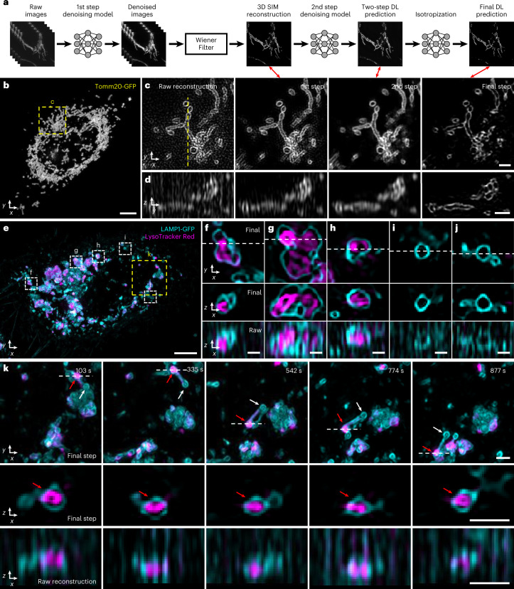
Fig. 5. Denoising and axial resolution enhancement facilitate 4D super-resolution imaging with isotropic resolution.
a, Schematic illustrating workflow for applying deep learning to raw input data. Sets of raw images (5 phases × 3 orientations) are denoised and combined with a generalized Wiener filter; and the resulting 3D SIM reconstruction is denoised and passed through our axial resolution enhancement workflow (Fig. 4a) to yield an isotropic, denoised, super-resolution prediction. See also Fig. 4a and Supplementary Figs. 14 and 17. b, Maximum intensity projection of final prediction for Tomm20-GFP label in a live U2OS cell, 25th timepoint from a 50-timepoint volumetric series. See also Supplementary Video 8. c, Single lateral plane corresponding to yellow dashed rectangular region in b, illustrating progressive improvement from 3D SIM reconstruction based on raw input data; after the first denoising model and Wiener filter; after applying the second denoising model; and after the isotropization model. Double-headed red arrows show corresponding steps in schematic a. d, As in b but for axial plane indicated by yellow dashed line in c. e, Maximum intensity projection of final prediction for live U2OS cells expressing lysosomal marker LAMP1-GFP (cyan) and additionally labeled with LysoTracker Red to mark the lysosome interior (magenta). First timepoint from a 60-timepoint volumetric series is shown. See also Supplementary Video 10. f–j, Higher magnification views of white dashed rectangular regions in e, illustrating lateral views (top), axial views along white dashed lines in lateral views (middle) and comparative axial views from 3D SIM reconstructions (bottom, ‘Raw’). k, Higher magnification view of yellow dashed rectangular region, emphasizing dynamics at selected timepoints. See also Supplementary Video 12. Top: lateral views, red arrow emphasizes lysosomal subregion filled by LysoTracker Red dye versus white arrow, indicating unfilled region; middle: axial view corresponding to white dashed lines; bottom: comparative 3D SIM axial view. Scale bars, 5 µm (b,e); 1 µm (c,d,k); and 500 nm (f–j). DL, deep learning; s, seconds.

