Figure 1:

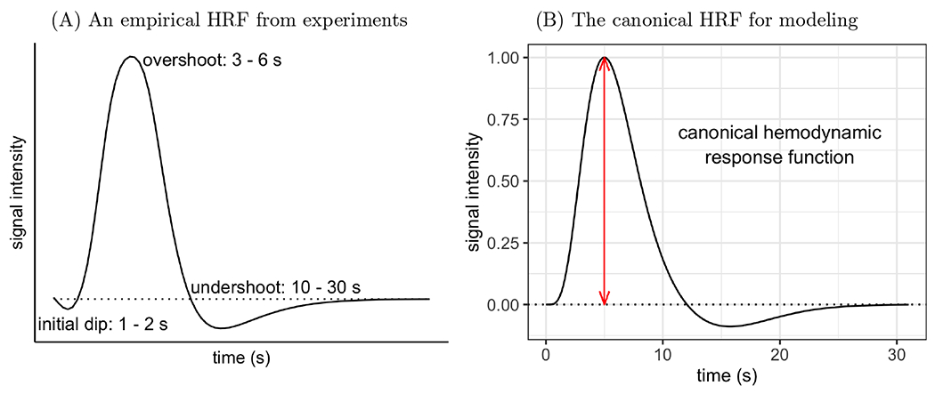
(A) Typical depiction of HRF shape and features based on FMRI and optical imaging experiments. The scale of the response intensity (vertical axis) depends on stimulus type, brain region, and local vasculature. (B) A canonical HRF for modeling (Friston et al., 1998) is usually constructed through an impulse response curve as a function of time t: here, h(t) = 5.7t⁵e^−t/Γ(6) – 0.95t¹⁵e^−t/Γ(16). It serves as a basis function and is convolved with stimulus timings to generate a series of expected HRFs for a task condition. These convolved HRFs are then used as regressors in a time series regression for acquired BOLD signals at the individual level. The overshoot peak occurs at 5 s and is scaled to 1 (red line) here. It is the sole focus in standard modeling, and the corresponding regression coefficient for a task condition with instantaneous trials can be conveniently interpreted as, for example, percent signal change. Moreover, the onset and duration of the undershoot are fixed, with a preset nadir of about 9% of the overshoot peak. The dotted horizontal line in both panels shows the baseline level of BOLD signal.