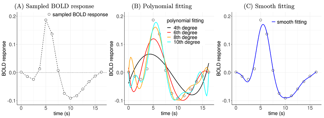
Figure 3:

Comparisons of fitting BOLD response data. (A) A hemodynamic response (in units of percent signal change), sampled at 14 points (empty circles) with a time resolution of 1.25 s, was estimated from an experimental participant through a regression model. The sampled values can be viewed with linear piecewise interpolation (dashed line). These points have a “jagged” appearance, even though they are sampled from a presumably smooth HRF. (B) Fitting the data with polynomials introduces some smoothness but is also usually challenging: even though higher-order polynomials fit better to the original data, they may poorly make out-of-sample predictions and introduce extraneous features. (C) Modeling the HRF with smooth splines (e.g., thin plates) intends to achieve a counterbalance between fitting and predictive accuracy.