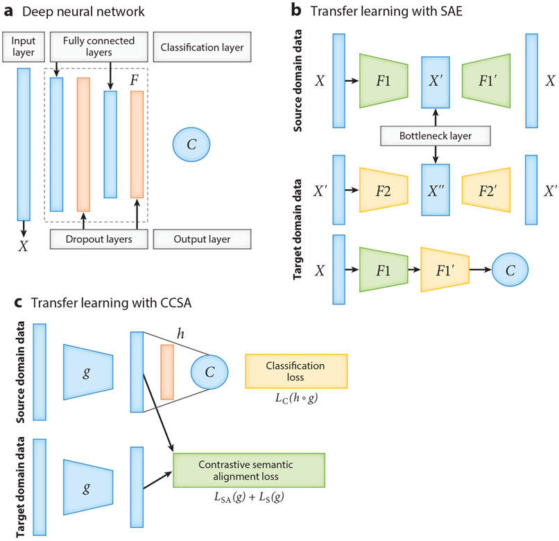
Figure 5.

The neural network architectures for deep learning and deep transfer learning. (a) An example architecture of a deep neural network model, which includes an input layer; several hidden layers (marked as $F$), including fully connected layers and dropout layers; and one output layer $C$. More fully connected layers can be added to the deep neural network model. (b) The neural network architecture of a stacked denoising auto-encoder (SAE) for transfer learning. $F1$ (or $F2$) is the encoder with two layers, including a fully connected layer and a dropout layer; $F{1}^{\prime }$ (or $F{2}^{\prime }$) is the decoder; the first and the second rows provide the structure of the first and second auto-encoders, respectively; and $C$ is a regression or classification layer. (c) The neural network architecture of classification and contrastive semantic alignment (CCSA) (105). CCSA minimizes the loss function $L_{\text{CCSA}}(f)=(1-\gamma )L_{\mathrm{C}}(b\circ g)+\gamma (L_{\text{SA}}(g)+L_{\mathrm{S}}(g))$, where $f=b\circ g$ represents the composition of a function $g$ that maps the input data $X$ to an embedding space $Z$ and a function $b$ used to predict the output label from $Z$; $C$ is a classification layer; $L_{\mathrm{C}}(b\circ g)$ is the classification loss; $L_{\text{SA}}(g)$ is the semantic alignment loss; $L_{\mathrm{S}}(g)$ is the separation loss; and $\gamma$ is the weight used to balance the classification loss versus the contrastive semantic alignment loss $L_{\text{SA}}(g)+L_{\mathrm{S}}(g)$.