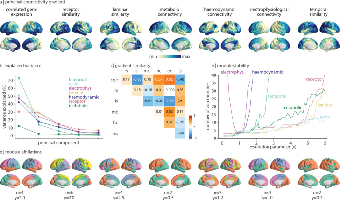
Fig 5. Gradients and modules of connectivity modes.

(a) The first principal component (“gradient”) of each connectivity mode is shown on the cortex. (b) The percent variance explained for the first 5 principal components of each connectivity mode. (c) The Pearson’s correlation between every pair of network gradients, visualized as a heatmap. CGE, correlated gene expression; RS, receptor similarity; LS, laminar similarity; MC, metabolic connectivity; HC, haemodynamic connectivity; EC, electrophysiological connectivity; TS, temporal similarity. (d) The Louvain community detection algorithm is applied to each connectivity mode across different resolution parameters (0.1 ≤ γ ≤ 6.0, in intervals of 0.1) and the number of ensuing communities is plotted as a function of γ. (e) For each connectivity mode, we show a single community detection solution for a specified γ, and we indicate the number of communities (n). The data underlying this figure can be found at https://github.com/netneurolab/hansen_many_networks.