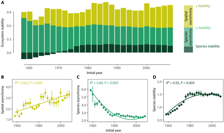
Fig. 2. Visualized temporal trends of species stability, species asynchrony, and spatial asynchrony over succession.

In (A), the widths of the shades represent the logarithm-transformed mean values of species stability (dark green), species asynchrony (bright green), and spatial asynchrony (dark yellow) within each 10-year time interval. Mathematically, at the logarithm-transformed scale, the α stability can be viewed as the sum of species stability and species synchrony, and the γ stability can be viewed as the sum of α stability and spatial synchrony. Spatial asynchrony (B) and species stability (D) significantly increased, but species asynchrony (C) significantly decreased over time. The x axis represents the initial year of each 10-year rolling window. Temporal trend lines were fitted using linear (B) and quadratic regression [(C) and (D)] that account for temporal autocorrelation, respectively.