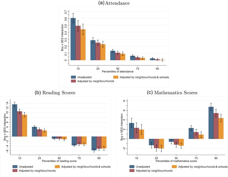
Fig. 4.

The Role of Schools and Neighbourhoods in the Gender Gap throughout the Distribution.

Note: The sample is individuals born between 1994 and 2000 in Florida, attending Florida public schools and having non-missing attendance and test score outcomes. These graphs plot the coefficients on the interaction of Boy × SES without additional Boy × other environmental factors (dark navy bars) as well as with the addition of the Boy × neighbourhood SES measure (medium maroon bars) or both Boy × neighbourhood SES measure and Boy × school quality (light orange bars). Each graph plots estimates from 15 unconditional quantile regressions, estimated using RIF regressions (Firpo et al., 2009) and implemented using the rifreg command in Stata. The quantiles of interest are 10, 25, 50, 75 and 90. Panel (a) presents results for attendance, panel (b) presents results for reading test scores and panel (c) presents results for mathematics test scores. Dependent variables are multiplied by 100. Estimates represented by dark navy bars come from regressing one of the three outcome variables on the Boy indicator, SES index, interaction between those two (plotted parameter of interest), school quality, neighbourhood SES index, race/ethnicity indicators, month-of-birth indicators, year-of-birth indicators and birth order indicators. Estimates represented by medium maroon bars include the same set of control variables, but further add Boy × neighbourhood SES index interaction. Estimates represented by light orange bars further add Boy × school quality interaction. Whiskers represent 95% confidence intervals based on bootstrapped SEs with 200 replications.